Excel scatter chart using text name

This Excel tutorial explains how to ordinal data (text) in scatter chart using bar chart.

Excel scatter chart using text name

Excel scatter chart requires the x axis and y axis for each data point to be plotted in a diagram, and then join all those point together to analyze the trend or analyze if x and y variables are correlated, where X and Y values have to be numeric values.

Below is an example showing how employee Grade is related to salary. From the graph, you can see the trend that Salary increases exponentially with Grade (although the data is dummy, the trend is real).

Sometimes we categorize x axis values as a group name (ordinal data) instead of providing the actual numeric value.

If we put text name in x axis (Grade), in order to force text name to become numeric, Excel converts first x value (Grade 1) to numeric value 1, the 2nd x value (Grade 3) to numeric value 2, and so on.  Therefore in the below scattered chart, we see 10 data points.

Solution – Excel scatter chart using text name

To group Grade text (ordinal data), prepare two tables:

1) Data source table

2) a mapping table indicating the desired order in X-axis

In Data Source table, vlookup up “Order” from “Mapping Table”,  we are going to use this Order value as x-axis value instead of using Grade.

In Mapping table, put a dummy 0 for Y axis.

Since Excel allows different chart types to be displayed in one chart, we are going to create a mix of bar chart (column chart) and scatter chart.

Scatter chart is used to display the actual data point, while bar chart is to display Grade labels.

– Create scatter chart for Range B20:C31 (Series 1)

– Add bar chart (column chart) for Range F20:G26 (Series 2)

Due to 0 y axis for Series 2, no value is displayed, only the x-axis label can be seen.

The outcome should look like below.

Alternatively, you can also create a another scattered graph for Series 2, then show x-value as label. However more steps are required.

Outbound References

http://superuser.com/questions/646759/scatter-chart-with-one-text-non-numerical-axis

Excel scatter chart using text name

Access BETWEEN timestamp problem

This Access tutorial explains the problem with BETWEEN timestamp, where the end date is not included in the result.

Access BETWEEN timestamp problem – end date not included

Very often you may receive data source that uses timeStamp (for example, 1/1/2015 15:34:00) instead of a Date (1/1/2015). The purpose of timestamp is to accurately record the time of action for auditing.

In Access (even other system), you may want to select data within specific date period, say, between 1/1/2014 and 1/1/2015. If the Field you want to apply criteria on is Date format, you can see results are able to correctly return both 1/1/2014 and 1/1/2015.

However, if you try to apply criteria between 1/1/2014 and 1/1/2015 to Field with timestamp, you will not be able to return any data on 1/1/2015.

To summarize the above:

When you use date criteria on two dates, both Begin Date and End Date are inclusive in the result.

When you use date criteria on two timestamp, End Date is not inclusive.

Reason – Access end date not included in BETWEEN timestamp

Use the same example as above.

When you apply criteria, between 1/1/2014 and 1/1/2015 on timestamp Field, Access needs to convert date to timestamp in order to do comparison. Because Access has no information what specific hh:mm:ss the date is, Access puts 00:00:00 in the date criteria.

Therefore the criteria between 1/1/2014 and 1/1/2015 is converted to between 1/1/2014 00:00:00  and 1/1/2015 00:00:00

After adding 00:00:00 to date, here comes the problem:

– If your database has a date which is 1/1/2014 01:00:00, it will return in the result because it is really between 1/1/2014 00:00:00  and 1/1/2015 00:00:00.

– If your database has a date which is 1/1/2015 01:00:00, it fails to return in the result because it is not between 1/1/2014 00:00:00  and 1/1/2015 00:00:00.

Solution- Access end date not included in BETWEEN timestamp

We have no problem using date in date Field because everything are considered 00:00:00. Similarly, to solve the timestamp issue, we can take away the hh:mm:ss part from timestamp.

To remove the time value, write an Expression as below

DateValue(TIMESTAMP)

See the below explanation for Access DateValue Function

Syntax of DateValue

DateValue ( date )

The required date argument is normally a string expression representing a date from January 1, 100 through December 31, 9999. However, date can also be any expression that can represent a date, a time, or both a date and time, in that range.

Outbound References

https://support.office.com/en-us/article/DateValue-Function-03878F08-B0DB-42DF-8A0C-279939637C6F

 

 

Access BETWEEN timestamp problem

Excel VBA Add Table AutoFilter cancel AutoFilter sorting

This Excel tutorial explains how to use Excel VBA to add Table AutoFilter, cancel Table AutoFilter, sorting Table

Excel VBA Add Table AutoFilter or Cancel AutoFilter

Using VBA to add AutoFilter or cancel Auto Filter is very simple if you know the code, but you should note that Excel does not treat Worksheet AutoFilter the same way as Table AutoFilter.

This article only talks about Table AutoFilter.

For Worksheet AutoFilter, click here.

Excel VBA Add Table AutoFilter

You can only have one Auto Filter in one Worksheet. However if you have Table, you can have one Worksheet Auto Filter, plus one Filter for each Table. AutoFilter in Table is an Object for each Table.

Table is a ListObjects, you can access the AutoFilter of Table by specifying Table name ListObjects(“Table_name”) or through ListObjects Array. If you have two Table in the worksheet, the first added Table is ListObjects(1) and the other is ListObjects(2).

Add Table AutoFilter

The below code add AutoFilter for ListObjects(1). If AutoFilter is already present, nothing will happen.

Dim LstObj As ListObject
Set LstObj = ActiveSheet.ListObjects(1)
LstObj.ShowAutoFilter = True

Cancel Table AutoFilter

The below code cancel AutoFilter for ListObjects(1). If AutoFilter is not present, nothing will happen.

Dim LstObj As ListObject
Set LstObj = ActiveSheet.ListObjects(1)
LstObj.ShowAutoFilter = False

Unhide filtered data

The below code unhide AutoFilter for ListObjects(1).

Dim LstObj As ListObject
Set LstObj = ActiveSheet.ListObjects(1) 
If LstObj.AutoFilter.FilterMode Then 
 LstObj.AutoFilter.ShowAllData 
End If

Apply criteria to Table AutoFilter

The syntax is exactly the same as Worksheet AutoFilter because both of them use AutoFilter Method of Range. the only difference is that you have to assess the Range Object of ListObject first.

The below example shows how to assess Range of LstObj in order to use AutoFilter Method.

LstObj.Range.AutoFilter Field:=1, Criteria1:=”A”, Operator:=xlOr, Criteria2:=”D”

Read the syntax of AutoFilter Method before you read on.

Name	Requiredl	Data Type	Description
Field	Optional	Variant	The integer offset of the field on which you want to base the filter (from the left of the list; the leftmost field is field one).
Criteria1	Optional	Variant	The criteria (a string; for example, “101”). Use “=” to find blank fields, or use “<>” to find nonblank fields. If this argument is omitted, the criteria is All. If Operator is xlTop10Items, Criteria1 specifies the number of items (for example, “10”).
Operator	Optional	XlAutoFilterOperator	One of the constants of XlAutoFilterOperator specifying the type of filter. Name Value Description xlAnd 1 Logical AND of Criteria1 and Criteria2. xlBottom10Items 4 Lowest-valued items displayed (number of items specified in Criteria1). xlBottom10Percent 6 Lowest-valued items displayed (percentage specified in Criteria1). xlFilterCellColor 8 Color of the cell xlFilterDynamic 11 Dynamic filter xlFilterFontColor 9 Color of the font xlFilterIcon 10 Filter icon xlFilterValues 7 Filter values xlOr 2 Logical OR of Criteria1 or Criteria2. xlTop10Items 3 Highest-valued items displayed (number of items specified in Criteria1). xlTop10Percent 5 Highest-valued items displayed (percentage specified in Criteria1).
Criteria2	Optional	Variant	The second criteria (a string). Used with Criteria1 and Operator to construct compound criteria.
VisibleDropDown	Optional	Variant	True to display the AutoFilter drop-down arrow for the filtered field. False to hide the AutoFilter drop-down arrow for the filtered field. True by default.

The below examples summarize all the basics you need to know about AutoFilter Criteria.

Example	Explanation
LstObj.Range.AutoFilter Field:=1, Criteria1:=”b”	Filter text criteria
LstObj.Range.AutoFilter Field:=1, Criteria1:=”b*”	Filter text criteria with Wildcard
LstObj.Range.AutoFilter Field:=2, Criteria1:=”>10″	Filter number criteria
LstObj.Range.AutoFilter Field:=1, Criteria1:=”b”, _ Operator:=xlOr, Criteria2:=”c”	Filter two text criteria using OR, which means the result shows b and c. Note that you can only have 2 criteria at most
LstObj.Range.AutoFilter Field:=1, Criteria1:= Array(“a”, “b”, “c”), Operator:=xlFilterValues	Filter two text criteria using Array
LstObj.Range.AutoFilter Field:=1, Criteria1:=”b” LstObj.Range.AutoFilter Field:=2, Criteria1:=”>10″	Filter two different Fields

Apply Table AutoFilter sorting

Before applying sorting, you should clear previous sorting first. To clear sorting in AutoFilter, use Sort.SortFields.Clear Method. Note that clear sorting does not reverse the data to the original order.

To tell AutoFilter how you want to sort the data, use Sort.SortFields.Add Method. (no data is sorted at this point)

Name	Required/Optional	Data Type	Description
Key	Required	Range	Specifies a key value for the sort.
SortOn	Optional	Variant	The field to sort on.
Order	Optional	Variant	Specifies the sort order.
CustomOrder	Optional	Variant	Specifies if a custom sort order should be used.
DataOption	Optional	Variant	Specifies the data option.

Finally, use Sort.Apply Method  to apply on the sort states.

The below example sorts data in Ascending Order in column A.

Dim LstObj As ListObject
Set LstObj = ActiveSheet.ListObjects(1)
LstObj.Sort.SortFields.Clear
LstObj.Sort.SortFields.Add Key:=Range("A:A"), SortOn:=xlSortOnValues, Order:=xlAscending, DataOption:=xlSortNormal
LstObj.Sort.Apply

Reset Table Filter

The below code unhide all hidden data and cancel sorting.

Dim LstObj As ListObject
Set LstObj = ActiveSheet.ListObjects(1)
LstObj.ShowAutoFilter = False
LstObj.ShowAutoFilter = True
LstObj.Sort.SortFields.Clear

 

Excel VBA Add Table AutoFilter cancel AutoFilter sorting

Excel VBA Add Autofilter Cancel AutoFilter sorting in worksheet

This Excel tutorial explains how to use Excel VBA to add AutoFilter, cancel AutoFilter, add sorting in Worksheet AutoFilter.

Excel VBA Add AutoFilter or Cancel AutoFilter

Using VBA to add AutoFilter or cancel Auto Filter is very simple if you know the code, but you should note that Excel does not treat Worksheet AutoFilter the same way as Table AutoFilter.

This article only talks about Worksheet AutoFilter.

Excel VBA AutoFilter in Worksheet

Add AutoFilter

AutoFilter is an Range Method. To add AutoFilter, you must specify the Cell which you want to add filter on. If you apply on A1, the Cells adjacent to A1 will have AutoFilter applied.

Range("A1").AutoFilter

You can specify which fields you need to apply AutoFilter to avoid adding AutoFilter applying on unwanted adjacent Cells.

Range("A1:A3").AutoFilter

Note that AutoFilter Method can also be used to cancel AutoFilter, if AutoFilter already exists.

Cancel AutoFilter

Because you can only have one AutoFilter in one Worksheet, you can check whether a Worksheet has AutoFilter using AutoFilterMode Property.

The below code cancel AutoFilter if found any.

If ActiveSheet.AutoFilterMode = True Then
   Range("A1").AutoFilter
End If

Unhide filtered data

You can use Worksheet Property FilterMode to check if there are filtered data in the worksheet. Use ShowAllData Method to unhide data.

If ActiveSheet.FilterMode = True Then
     ActiveSheet.ShowAllData
End If

Apply criteria to AutoFilter

Read the syntax of AutoFilter Method before you read on.

Name	Required/Optional	Data Type	Description
Field	Optional	Variant	The integer offset of the field on which you want to base the filter (from the left of the list; the leftmost field is field one).
Criteria1	Optional	Variant	The criteria (a string; for example, “101”). Use “=” to find blank fields, or use “<>” to find nonblank fields. If this argument is omitted, the criteria is All. If Operator is xlTop10Items, Criteria1 specifies the number of items (for example, “10”).
Operator	Optional	XlAutoFilterOperator	One of the constants of XlAutoFilterOperator specifying the type of filter. Name Value Description xlAnd 1 Logical AND of Criteria1 and Criteria2. xlBottom10Items 4 Lowest-valued items displayed (number of items specified in Criteria1). xlBottom10Percent 6 Lowest-valued items displayed (percentage specified in Criteria1). xlFilterCellColor 8 Color of the cell xlFilterDynamic 11 Dynamic filter xlFilterFontColor 9 Color of the font xlFilterIcon 10 Filter icon xlFilterValues 7 Filter values xlOr 2 Logical OR of Criteria1 or Criteria2. xlTop10Items 3 Highest-valued items displayed (number of items specified in Criteria1). xlTop10Percent 5 Highest-valued items displayed (percentage specified in Criteria1).
Criteria2	Optional	Variant	The second criteria (a string). Used with Criteria1 and Operator to construct compound criteria.
VisibleDropDown	Optional	Variant	True to display the AutoFilter drop-down arrow for the filtered field. False to hide the AutoFilter drop-down arrow for the filtered field. True by default.

The below examples summarize all the basics you need to know about AutoFilter Criteria.

Example	Explanation
Range(“A1″).AutoFilter Field:=1, Criteria1:=”b”	Filter text criteria
Range(“A1″).AutoFilter Field:=1, Criteria1:=”b*”	Filter text criteria with Wildcard
Range(“A1″).AutoFilter Field:=2, Criteria1:=”>10″	Filter number criteria
Range(“A1″).AutoFilter Field:=1, Criteria1:=”b”, _ Operator:=xlOr, Criteria2:=”c”	Filter two text criteria using OR, which means the result shows b and c. Note that you can only have 2 criteria at most
Range(“A1″).AutoFilter Field:=1, Criteria1:= Array(“a”, “b”, “c”), Operator:=xlFilterValues	Filter two text criteria using Array
Range(“A1″).AutoFilter Field:=1, Criteria1:=”b” Range(“A1″).AutoFilter Field:=2, Criteria1:=”>10″	Filter two different Fields

Apply AutoFilter sorting

Before applying sorting, you should clear previous sorting first. To clear sorting in AutoFilter, use Sort.SortFields.Clear Method. Note that clear sorting does not reverse the data to the original order.

To tell AutoFilter how you want to sort the data, use Sort.SortFields.Add Method. (no data is sorted at this point)

Name	Required/Optional	Data Type	Description
Key	Required	Range	Specifies a key value for the sort.
SortOn	Optional	Variant	The field to sort on.
Order	Optional	Variant	Specifies the sort order.
CustomOrder	Optional	Variant	Specifies if a custom sort order should be used.
DataOption	Optional	Variant	Specifies the data option.

Finally, use Sort.Apply Method  to apply on the sort states.

The below example sorts data in Ascending Order in column A.

ActiveSheet.AutoFilter.Sort.SortFields.Clear
ActiveSheet..AutoFilter.Sort.SortFields.Add Key:=Range ("A:A"), SortOn:=xlSortOnValues, Order:=xlAscending, DataOption:= xlSortNormal
ActiveSheet..AutoFilter.Sort.Apply

Reset Filter

This is a summary of all the above tutorials. Unhide all hidden data and cancel sorting.

If ActiveSheet.AutoFilterMode = False Then
   Range("A1").AutoFilter
Else 
 ActiveSheet.AutoFilter.Sort.SortFields.Clear
 If ActiveSheet.FilterMode = True Then
     ActiveSheet.ShowAllData
 End If
End If

Excel VBA Add Autofilter Cancel AutoFilter sorting in worksheet

Tips on Microsoft Office Specialist for Excel exam MOS

What is Microsoft Office Specialist for Excel exam?

Microsoft Office Specialist (also known as MOS) is a certificate that can be earned if you pass an exam.

Microsoft Office Specialist has exams for different Office products, which include Microsoft Word, Powerpoint, Excel, Access, Outlook, SharePoint, OneNote. Microsoft Word and Excel are slightly different, each of them have two levels, one is Core level and the other is Expert level.

If you take a specific combination of exams, you can earn an additional certificate called “Microsoft Office Specialist Master”. Since the combination may change over time, please refer to Microsoft Homepage for details.

https://www.microsoft.com/learning/en-us/mos-certification.aspx

Why should I take Microsoft Office Specialist for Excel exam?

I am sharing the reason as a HR professional. Some may argue certificate is useless, you can have lots of certificates but you may not have the skills or experience, I will tell you why it is not true.

If you apply for a job, 99.9% time you need to go through a HR recruiter first for screening, but most recruiters do not have Excel skills, not to say to evaluate whether you are good at Excel. Work experience is one of the things recruiter would use to guess the level of your Excel skills, but it is not reliable because your skills may only focus on one particular area relevant to the job. If your job relies on Excel very much, they may give you an Excel test but most companies would not do that because it is time wasting and they don’t have the knowledge to make a decent test.

Given that two applicants have similar work experience, when a recruiter makes a decision which candidate to refer to line manager, they would definitely choose the one with Excel certificate, why? Because if you really suck at Excel after you are hired, the recruiter can justify his decision, line manager cannot blame him. Now you know why certificate is important.

How to take Microsoft Office Specialist for Excel exam

Microsoft corporates with Certiport to arrange the exam, you can find a Certiport exam center near you to take the exam.

Before you take the exam, you have to register an account in Certiport, and then call the desired exam center to book an exam time and pay the exam fee of about $80 USD. Sometimes there is promotion for your to retake the exam if fail.

Upon completion of the exam, you will immediately know your score and the passing score, and the exam center staff will print a hardcopy of the exam result to you.

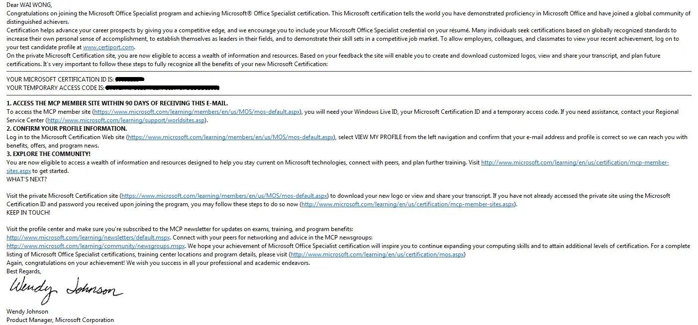
Microsoft will send you a confirmation email within several weeks later, from my experience it took 2 days.

Note that Certiport is now responsible for the administration of certificate. To view the eCert and request hard copy:

1) Logon to Certiport

2) Navigate to MyCertiport > My Transcript > Select View Mode “Personal View”

3) Click on “PDF” to download eCert. You can also pay $10USD plus $5 for shipping fee to delivery hard copy certificate.

MOS Excel Core or MOS Excel Expert?

As I mentioned earlier, there are two levels of MOS Excel exam, one is Core and one is Expert (if Expert is not mentioned, then it is Core). If you are going for the MOS Master certificate, you have to take Excel Expert exam. If you are just looking to earn a certificate for employment purpose, you don’t need to take Expert, because I am sure 99% employers have not heard about MOS Excel exam, not to say they know there are two levels for the Excel exam.

Sharing on Microsoft Office Specialist for Excel exam

Recently, I took the exam 77-882: MOS: Microsoft Office Excel 2010 and passed the exam. If you are interested in taking the exam as well, you have come to the right place, as I can’t find any sharing from google or yahoo. I can only search articles that say “it is easy”, but it doesn’t help.

Unlike many other IT certificates which are multiple choice exams, MOS Excel is a practical exam which requires you to perform tasks in the simulated Excel environment. I must remind you that you cannot trust any brain dump for this MOS Excel exam, especially those with 50 something questions pool which I think is unbelievable.

Preparing MOS: Microsoft Office Excel 2010

As a student, you must have experience taking public examinations and you prepare your exams by reading past paper, in which you can learn how the questions are asked. For MOS exam, just buy a book, you will not find the exact same question from the book but a book shows you step by step how to perform a task and it covers all contents in the syllabus, therefore you will find many questions are highly similar to the real exam questions. Don’t bother which book to buy if you find more than one, as most of them have very similar contents.

I suggest you to buy a book from bookstore, ebook has no quality control and you cannot preview the book first. One of the reasons I didn’t take Expert level is that I couldn’t find any book for Expert level from bookstore.

If you don’t want to buy a book, I am sure you can still pass the exam if you know Excel well, you just need some hints on the scope of exam. In my exam, there were 16 questions, each question comprised two tasks (which can be considered as 32 questions, as two parts are irrelevant). You need to score at least 700/1000 marks to pass the exam but Microsoft would not tell how the scoring system works. You have 45 minutes to complete the questions, you can skip the questions and come back later.

Below is the scope of the exam that I copied from Microsoft website, I will highlight the items that actually appeared in my exam. You will find one item highlighted in each line of the syllabus.

Managing the worksheet environment

• Navigate through a worksheet
  
  
  

  • Hot keys, name box
  
  
  
  


• Print a worksheet or workbook
  
  
  

  • Printing only selected worksheets; printing an entire workbook; constructing headers and footers; applying printing options (scale, print titles, page setup, print area, gridlines)
  
  
  
  


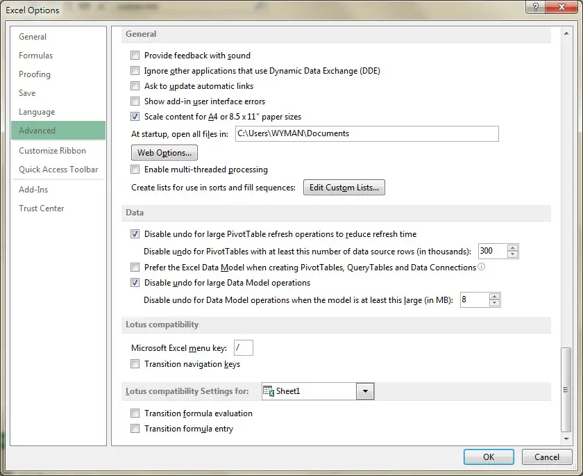
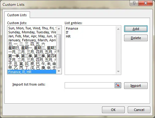
• Personalize environment by using Backstage
  
  
  

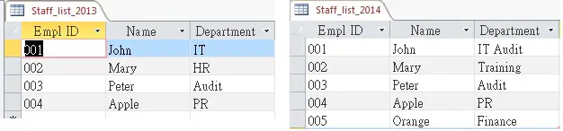
  • Manipulating the Quick Access toolbar; manipulating the ribbon tabs and groups; manipulating Excel default settings; importing data to Excel; importing data from Excel; demonstrating how to manipulate workbook properties; manipulating workbook files and folders; applying different name and file formats for different uses by using Save and Save As features
  
  
  
  

Creating cell data

• Construct cell data
  
  
  

  • Using paste special (formats, formulas, values, preview icons, transpose rows and columns, operations, comments, validation, paste as a link); cutting, moving, and selecting cell data
  
  
  
  


• Apply AutoFill
  
  
  

  • Copying data using AutoFill; filling series using AutoFill; copying or preserving cell format with AutoFill; selecting from drop-down list
  
  
  
  


• Apply and manipulate hyperlinks
  
  
  

  • Creating a hyperlink in a cell; modifying hyperlinks; modifying hyperlinked-cell attributes; removing a hyperlink
  
  
  
  

Formatting cells and worksheets

• Apply and modify cell formats
  
  
  

  • Aligning cell content; applying a number format; wrapping text in a cell; using Format Painter
  
  
  
  


• Merge or split cells
  
  
  

  • Using Merge & Center, Merge Across, Merge Cells, and Unmerge Cells
  
  
  
  


• Create row and column titles
  
  
  

  • Printing row and column headings; printing rows to repeat with titles; printing columns to repeat with titles; configuring titles to print only on odd or even pages; configuring titles to skip the first worksheet page
  
  
  
  


• Hide and unhide rows and columns
  
  
  

  • Hiding a column; unhiding a column; hiding a series of columns; hiding a row; unhiding a row; hiding a series of rows
  
  
  
  


• Manipulate page setup options for worksheets
  
  
  

  • Configuring page orientation; managing page scaling; configuring page margins; changing header and footer size
  
  
  
  


• Create and apply cell styles
  
  
  

  • Applying cell styles; constructing new cell styles
  
  
  
  

Managing worksheets and workbooks

• Create and format worksheets
  
  
  

  • Inserting worksheets; deleting worksheets; copying, repositioning, copying and moving, renaming, grouping; applying coloring to worksheet tabs; hiding worksheet tabs; unhiding worksheet tabs
  
  
  
  


• Manipulate window views
  
  
  

  • Splitting window views; arranging window views; opening a new window with contents from the current worksheet
  
  
  
  


• Manipulate workbook views
  
  
  

  • Using Normal, Page Layout, and Page Break workbook views; creating custom views
  
  
  
  

Applying formulas and functions

• Create formulas
  
  
  

  • Using basic operators; revising formulas
  
  
  
  


• Enforce precedence
  
  
  

  • Order of evaluation, precedence using parentheses, precedence of operators for percent vs. exponentiation
  
  
  
  


• Apply cell references in formulas
  
  
  

  • Relative, absolute
  
  
  
  


• Apply conditional logic in a formula
  
  
  

  • Creating a formula with values that match your conditions; editing defined conditions in a formula; using a series of conditional logic values in a formula
  
  
  
  


• Apply named ranges in formulas
  
  
  

  • Defining, editing, and renaming a named range
  
  
  
  


• Apply cell ranges in formulas
  
  
  

  • Entering a cell range definition in the formula bar; defining a cell range using the mouse; defining a cell range using a keyboard shortcut
  
  
  
  

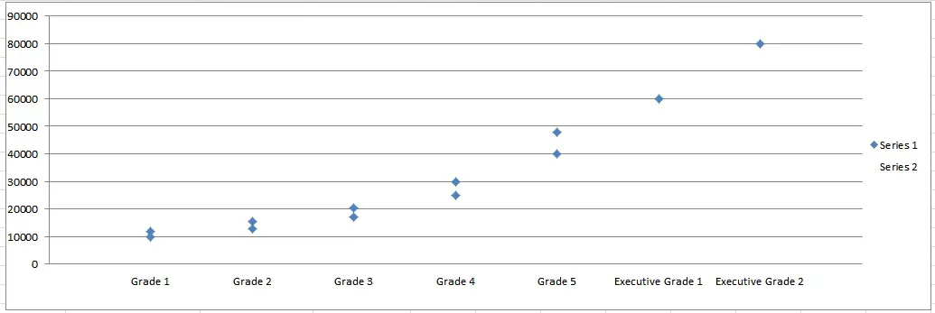
Presenting data visually

• Create charts based on worksheet data


• Apply and manipulate illustrations
  
  
  

  • Clip Art, SmartArt, shapes, screenshots
  
  
  
  


• Create and modify images by using the Image Editor
  
  
  

  • Making corrections to an image (sharpening or softening an image, changing brightness and contrast); using picture color tools; changing artistic effects on an image
  
  
  
  


• Apply Sparklines
  
  
  

  • Using Line, Column, and Win/Loss chart types; creating a Sparkline chart; customizing a Sparkline; formatting a Sparkline; showing or hiding data markers
  
  
  
  

Sharing worksheet data with other users

• Share spreadsheets by using Backstage
  
  
  

  • Sending a worksheet via email or OneDrive; changing the file type to a different version of Excel; saving as PDF or XPS
  
  
  
  


• Manage comments
  
  
  

  • Inserting, viewing, editing, and deleting comments
  
  
  
  

Analyzing and organizing data

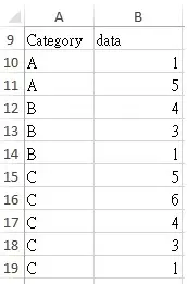
• Filter data
  
  
  

  • Defining, applying, removing, searching, filtering lists using AutoFilter
  
  
  
  


• Sort data
  
  
  

  • Using sort options (values, font color, cell color)
  
  
  
  


• Apply conditional formatting
  
  
  

  • Applying conditional formatting to cells; using the Rule Manager to apply conditional formats; using the IF Function and Apply Conditional Formatting, icon sets, data bars, clear rules
  
  
  
  

Conclusion of Microsoft Office Specialist for Excel exam

Before the exam, I bought a book for MOS Excel exam for about $20 USD, I did not look at the syllabus above, I only spent about 2 hours on the book in total. I quickly scanned through the book and I thought the exam was easy although there were features I had never used before.

In the exam, I had only one part of one question I was not sure about, the other questions were not difficult and even if I had never used some features before, the question clearly told me the name of the action so I could easily found the button, but it took me some time to find the button.

In the 45 minutes exam, I spent 35 minutes to complete all 16 questions, which is apparently not efficient. I suggest you to try everything in the syllabus at home and that will save you some time searching the buttons and trying the function.

And finally my score is … 800/1000, which is pretty close to the passing score 700/1000,  but I only got 1 part of question I was not sure. After the exam, I read another Access book I bought for MOS Access, the author captured the screen of the examination guideline at the beginning of the computer test, the guideline says that some questions only see the final result, while some would also see how you do it. I think this rule also applies to MOS Excel, therefore you need to reset the question if your answer is not one-shot.

To conclude:

For Excel novice: If you do not always use Excel, take a course. If you type “Microsoft Office Specialist” in search engine, you will find some local training centers that offer this course. If your course is customized for specific certificate, the trainer usually gives a set of questions for you which could be highly similar to the exam questions.

For Excel intermediate: If you use Excel on daily basis but only explore 50% of the Excel functions, don’t take any course. Go to bookstore and buy a book to self study and make sure you are familiar with everything in the syllabus

For Excel pro: If you use Excel on daily basis and you have explored 90% of the Excel functions (no VBA is required), you just need to scan through the syllabus and focus on the functions you don’t know in the syllabus, practice once before the exam and you are good to go.

I hope my experience will help you better prepare the exam, good luck~

 

Tips on Microsoft Office Specialist for Excel exam MOS

Excel use If condition on aggregate Function using Array

This Excel tutorial explains how to use If condition on aggregate Function using Array such as Average, Median, Mean, Maximum, Minimum.

Excel use If condition on aggregate Function using Array

Some Excel formula require you to input a range cells as argument in order to calculate a value, such as Sum, Count, Average, Median, Mean, Maximum, Minimum.

However, in those formula, you cannot use If Condition on the data Range before calculating Sum, Count, Average, Median, Mean, Maximum, Minimum.

For example, the below Function will not work correctly

=SUM(IF(A10:A19="A",B10:B19))

Example – Use Array to apply IF condition on Sum, Median

Use the below data as an example.

If you try to sum the data for Category A, you can apply SUMIF.

However, there is an alternative way to do that using Array.

=SUM(IF(A10:A19="A",B10:B19))

In the above formula, the brackets represent Array. Array does not work if you type directly in keyboard. After typing the formula inside , press CTRL+SHIFT+ENTER to turn the formula  into Array, will be added automatically.

Instead of evaluating whether A10:A19=”A” as a whole, Array evaluates whether A10=”A”, A11=”A”,A12=”A”, A13=”A”… individually and return the respective B10:B19 value if TRUE, finally Sum all the returned numbers.

Below is the evaluation process of Array:

=SUM(IF(A10:A19="A",B10:B19))
=SUM(IF(TRUE;TRUE;FALSE;FALSE;FALSE;FALSE;FALSE;FALSE;FALSE;FALSE,B10:B19))
=SUM(1,5)
=6

Similarly, you can apply If Condition on other statistical Functions or aggregate Functions. Take Median as another example.

To find the Median of Category A

=MEDIAN(IF(A10:A19="A",B10:B19))
=MEDIAN(IF(TRUE;TRUE;FALSE;FALSE;FALSE;FALSE;FALSE;FALSE;FALSE;FALSE,B10:B19))
=MEDIAN(1,5)
=3

To find the Maximum of Category B

=MAX(IF(A10:A19="B",B10:B19))
=MAX(IF(FALSE;FALSE;TRUE;TRUE;TRUE;FALSE;FALSE;FALSE;FALSE;FALSE,B10:B19))
=MAX(4,3,1)
=3

You can even combine AND / OR to evaluate in Array

=MAX(IF(OR(A10:A19="C",A10:A19="B"),B10:B19)

Outbound References

https://www.youtube.com/watch?v=DSivs93UDgc

 

Excel use If condition on aggregate Function using Array

Access count substring in string or text

This Access tutorial explains how to count substring in string (text).

Access count substring in string (text)

Access does not have a buit-in Function to count substring in string (text), instead you need to work around to get the job done. Alternatively, I have made a VBA solution for your reference.

Access count substring in string using Len and Replace Function

Access Len Function is to measure the length of text.

Access Replace Function is to replace a substring in a text.

To count substring in string, simply replace the target substring with nothing (removing the substring), and then measure the difference of text length before and after replace, and then divide the difference by length of substring.

For example, [str] field contains the string, while [substr] field is the substring.

 (Len([str])-Len(Replace([str],[substr],"")))/Len([substr])

Access VBA custom Function to count substring in string

I created this custom Function long time ago before I knew the Len and Replace trick, now this is for your reference.

Public Function wCountSubStr(str As String, substr As String) As Integer
    lenstr = Len(str)
    lensubstr = Len(substr)
    
    For i = 1 To lenstr
        tempString = Mid(str, i, lensubstr)
        If tempString = substr Then
            count = count + 1
        End If
    Next i
    wCountSubStr = count
End Function

Syntax of Custom Function – count substring in string

wCountSubStr(str, substr)

str	String to be evaluated
substr	Substring that you want to count

Example of Custom Function – count substring in string

Formula	Result
wCountSubStr(“123412″,”12″)	2
wCountSubStr(“#**$”,”1″)	0

 

Access count substring in string or text

Excel count substring in string or text

This Excel tutorial explains how to count substring in string (text).

Excel count substring in string (text)

Excel does not have a buit-in Function to count substring in string (text), instead you need to work around to get the job done. Alternatively, I have made a Macro solution for your reference.

Excel count substring in string using Len and Substitute Function

Excel Len Function is to measure the length of text.

Excel Substitute Function is to replace a substring in a text.

To count substring in string, simply replace the target substring with nothing (removing the substring), and then measure the difference of text length before and after substitute, and then divide the difference by length of substring.

For example, A1 contains the string, while B1 is the substring.

=(LEN(A1)-LEN(SUBSTITUTE(A1,B1,””)))/LEN(B1)

Excel VBA custom Function to count substring in string

I created this custom Function long time ago before I knew the Len and Substitute trick, now this is for your reference.

Public Function wCountSubStr(str As String, substr As String) As Integer
    lenstr = Len(str)
    lensubstr = Len(substr)
    
    For i = 1 To lenstr
        tempString = Mid(str, i, lensubstr)
        If tempString = substr Then
            count = count + 1
        End If
    Next i
    wCountSubStr = count
End Function

Syntax of Custom Function – count substring in string

wCountSubStr(str, substr)

str	String to be evaluated
substr	Substring that you want to count

Example of Custom Function – count substring in string

Formula	Result
=wCountSubStr(“123412″,”12″)	2
=wCountSubStr(“#**$”,”1″)	0

 

Excel count substring in string or text

Compare difference between two tables in MS Access Query

This Access tutorial explains how to compare difference between two tables in MS Access Query

Compare difference between two tables in MS Access Query

Access does not have a built-in Function to compare difference, but since we can write SQL and design Query in Access, we can make use of the properties of SQL JOIN to compare difference.

There are three kinds of JOIN in SQL – Inner Join, Left Join, Right Join.

Assume that you have two tables, table1 and table2, where you join them using a key Field “Employee ID”.

Inner Join

Return rows that have the common Employee ID in both tables

Left Join (Left Outer Join)

Return all rows in table1, plus fields in table2 where the Employee ID are matched (same as Excel vlookup, using table1 as a base, and then vlookup the employee ID in table2 for the required field)

In Excel, if table1 fails to vlookup key from table2, #N/A is returned. In Access, those #N/A data are known as Null value.

The whole point of Left Join is to find out those fields containing Null value, then we know what keys are present in table1 but not present in table2.

Right Join (Right Outer Join)

Same as Left Join, except that table1 becomes table2, table2 becomes table1. (using table2 as a base, and then vlookup the employee ID in table1 for the required field)

Excel Vlookup vs Access Query, which one is better for data comparison?

If your job requires to compare difference frequently, think about Access.

Factors considered in data comparison	Excel	Access
Performance dealing with mass data		Win
Performance dealing with mass formula		Win
Handling multiple keys for matching		Win
Time required to build comparison Query/Formula		Win
Accuracy of handling Null data		Win
Look for mistakes made in Query/Formula		Win
File size		Win
Re-usability of comparison template		Win

Example – compare difference between two tables

Assume that we have 2 staff lists, one is 2013 and the other is 2014. During the year, some employees have transferred to another department. Now we want to compare difference between these two tables.

Create a query in Query Design.

Add the two tables that we need to compare

To fully compare the queries, we need to make 3 comparisons. (In Excel, we vlookup in both sides to find out the variance)

1) Which records are completely the same

2) Which records exist in 2013 but not 2014

3) Which records exist in 2014 but not 2013

Records that are completely the same

In the Query Design, create an Inner Join (a straight line across two fields) for the key fields (say, Empl ID and Name) and fields you need to compare (Department). To create a join, simply drag from 2013 field over 2014 field.

The result will show records where 3 fields are exactly identical.

Records exist in 2013 but not 2014

Based on the last Query, double click on the first line between two tables.

Select the second option to create Left Join.

Repeat the above steps for the other two lines. Now the lines turn into arrows pointing from left to right, indicating it is a Left Join.

Click Run to see the result.

All 2013 data are present in the result, and we try to lookup the data from 2013 to see whether we can find the Empl ID+Name+Department key in 2014.

In Vlookup concept, those blank values are #N/A value (known as Null value in SQL)

Add criteria Is Null for 2014 Empl ID

Press Run, the result shows data containing Null 2014 Empl ID, that is the difference you are looking for.

Records exist in 2014 but not 2013

Repeat the steps in Left Join, except that we select the third option in Join Property.

This time the arrows point to the left, and then add criteria Is Null for 2013 Empl ID

Press Run to see result.

Outbound References

http://www.techonthenet.com/sql/joins.php

 

Compare difference between two tables in MS Access Query

Access error Type Num Div/0 Num

This tutorial explains the cause of Access errors in Access Query, Report, Form. These include #Error #Type! #Num! #Div/0! #Name.

Access error #Error #Type! #Num! #Div/0! #Name

There are several very common errors you may encounter in Access Query, Report or Form. It is very useful to understand the error in order to fix it, otherwise you will need to spend a lot of time to find out what Access is trying to tell you.

Access error #Error!

Access error #Error! occurs in an Expression where you try to do calculation on two Fields, however, Access cannot recognize one of them (or both of them) is Number so Access fails do a calculation.

For example, you cannot calculate Apple+1, because Apple is a Text.

Note that even if your Field is a Text, as long as the data is a number, Access can still do calculation.

Access error #Num!

There are many reasons that can cause Access #Num! error, below are two popular reasons.

Linked Table

In Linked Table, Access uses the first 8 rows of data to determine the data type of the Field. If Access sees the first 8 are Numbers, the data type is determined to be Number, but if you input Text in the 9th row, #Num! error occurs for that data.

Expression

If you divide 0 by 0, #Num! error occurs.

To solve the problem, use iff in Expression to capture this scnerio

iif(value1 = 0 AND value 2=0, 0, value1/value2)

Access error #Div/0!

If you divide a value by 0, #Div/0! occurs.

To solve the problem, use iff in Expression to capture this scenario

iif(value2 = 0,"your message", value1/value2)

For some calculations, this error is meaningful and should remain.

For example, if you are calculating an employee turnover rate

(number of leavers) / (headcount)

The headcount 0 has special implication and you should be alerted.

Access error #Type!

Access error #Type! occurs when two different Objects are used in a calculation, which means Access cannot recognize you are calculating two Numbers, Access thinks you are calculating a Table, a Query etc with a Number. This error is most likely caused by using inappropriate naming of the Fields, you should carefully note the Fields you use in calculation is not same as other Controls, such as Text Box name. If you can’t find any, perhaps you are using reserved name in Access.

For example, you should not name a Field as “Name”, because it is a reserved word referring to other Objects.

Click here to find out the list of reserved words.

You can either avoid using reserved words in Report/Form, or you can do your calculation in Query first.

Access error #Name

The cause of #Name Error is very similar to that of #Type! error. Below are three main reasons for #Name error.

Circular Reference

Field name is same as Control name (such as Text Box name). Access is confused whether to refer to the Field or Control, you should rename your Field or Control.

Reserved Word

Access has some reserved words that you should not use as field name.

Click here to find out the list of reserved words.

Data not updated

Access may not recognize the latest version of your data source, therefore Access cannot find the newly added Field name your are referring to in the source.

To refresh the data source, change data source to another table, and then change back to the data source.

Access error Type Num Div/0 Num

Access Report keep a group together in one page

This Access tutorial explains how to keep a group together in one page in Access Report.

Access Report – keep a group together in one page

In Access Report, you can group a Field and then display the grouping in Group Header, and display the value in Details. Sometimes the Details may be so long that it extends to the next page, breaking up the same group into two pages. Access Report has a function called “group together in one page” to cope with this issue.

Access Report Example – keep a group together in one page

Assume that you have a staff list with two fields – Department and staff name. After grouping the data by Department in Access Report, you see the followings in Print Preview.

———————————–

Page 1:

Department A

Staff1

Staff2

Staff3

Staff4

Department B

Staff5

———————————–

Page 2:

Staff6

Staff7

Department C

Staff 8

Staff 9

———————————–

In page 1, you can see that staff in Department B are separated in two pages.

To fix this, at the Group, Sort, and Total Section, choose the option keep whole group together on one page. This will force Department B to start a new page.

Access Report Result – keep a group together in one page

Now you will see the result looks like this.

———————————–

Page 1:

Department A

Staff1

Staff2

Staff3

Staff4

———————————–

Page 2:

Department B

Staff5

Staff6

Staff7

Department C

Staff 8

Staff 9

———————————–

Explanation of Result – keep a group together in one page

First of all, Department B starts a new page as expected, starting in a new page.

Second, Department C did not start in a new page because its data is not extended to Page 3, so Department C already successfully keeps the group together in one page, no change is needed.

If you want to start a new page for each department, click on the Department Header in the design view > Properties > Force New Page > select “Before Section”

Outbound References

http://www.experts-exchange.com/Database/Reporting/Crystal_Reports/Q_28174740.html

Access Report keep a group together in one page

Excel VBA Rnd Function to generate random number

This Excel tutorial explains how to use Excel VBA Rnd Function to generate random number and create custom Function for random decimal number.

Excel VBA Rnd Function to generate random number

Rnd Function is for use in Access, Access VBA, Excel VBA, it is used to generate random number larger than 0 and smaller than 1 (1 and 0 exclusive).

Excel worksheet use RAND Function and RANDBETWEEN Functions, which have quite different behavior.

Syntax of Excel VBA Rnd Function

Rnd[(number)]

Number	Rnd generates
Not supplied or any positive number	Generate a new random number
0	Return the last generated number
Any negative number	Generate a new random number and use it every time

Example of Excel VBA Rnd Function – generate random number

It is not useful to use Excel VBA Rnd Function alone, because we ultimately want to generate a random number between two specific numbers, but not a random number between 0 and 1.

Use the below formula to generate a number bounded by lowerbound and upperbound (both inclusive).

Int ((upperbound - lowerbound + 1) * Rnd + lowerbound)

Formula	Explanation
Int((10-1+1)*Rnd()+1)	Generate random number between 1 and 10
Int((200-100+1)*Rnd()+100)	Generate random number between 100 and 200

VBA Function – generate random decimal number

If you think the formula is too complicated, you can use the below custom Function. The purpose of this custom Function is to simulate Excel worksheet Function RandBetween, which allows you to simply use upperbound and lowerbound as Function arguments.

This custom Function offers an optional parameter that allows you to generate random integer or decimal number.

VBA code of custom Function – generate random decimal number

Public Function wRandomNumber(lowerbound, upperbound, Optional rndType = 1) As Double
 Randomize
    rndVariable = Rnd
    If rndType = 1 Then
        wRandomNumber = Int((upperbound - lowerbound + 1) * rndVariable + lowerbound)
    ElseIf rndType = 2 Then
        If (upperbound - lowerbound + 1) * rndVariable + lowerbound <= upperbound Then
            wRandomNumber = (upperbound - lowerbound + 1) * rndVariable + lowerbound
        Else
            Do While (upperbound - lowerbound + 1) * rndVariable + lowerbound > upperbound
                rndVariable = Rnd
                If (upperbound - lowerbound + 1) * rndVariable + lowerbound <= upperbound Then
                    wRandomNumber = (upperbound - lowerbound + 1) * rndVariable + lowerbound
                End If
            Loop
        End If
    End If
End Function

Syntax of custom Function – generate random decimal number

wRandomNumber(lowerbound, upperbound, [rndType])

lowerbound	The minimum random number
upperbound	The maximum random number
rndType	Optional, indicate whether the random number is decimal or integer value description 1 (default) Return a random integer 2 Return a random decimal number

Example of custom Function – generate random decimal number

Formula	Explanation
=wRandomNumber(1,100)	Return a random integer between 1 and 100 (both inclusive)
=wRandomNumber(100,200,2)	Return a random decimal number between 100 and 200 (both inclusive)

Outbound References

https://support.office.com/en-us/article/Rnd-Function-503CD2E4-3949-413F-980A-ED8FB35C1D80

Excel VBA Rnd Function to generate random number

Access Rnd Function generate random number and decimal

This Access tutorial explains how to use Access Rnd Function to generate random number and create custom Function for random decimal number.

Access Rnd Function to generate random number

Access Rnd Function is for use in Access, Access VBA, Excel VBA, it is used to generate random number larger than 0 and smaller than 1 (1 and 0 exclusive).

Syntax of Access Rnd Function

Rnd[(number)]

Number	Rnd generates
Not supplied or any positive number	Generate a new random number
0	Return the last generated number
Any negative number	Generate a new random number and use it every time

Example of Access Rnd Function – generate random number

It is not useful to use Rnd Function alone, because we ultimately want to generate a random number between two specific numbers, but not a random number between 0 and 1.

Use the below formula to generate a number bounded by lowerbound and upperbound (both inclusive).

Int ((upperbound - lowerbound + 1) * Rnd + lowerbound)

Formula	Explanation
Int((10-1+1)*Rnd()+1)	Generate random number between 1 and 10
Int((200-100+1)*Rnd()+100)	Generate random number between 100 and 200

Access VBA Function – generate random decimal number

If you think the formula is too complicated, you can use the below custom Function. The purpose of this custom Function is to simulate Excel worksheet Function RandBetween, which allows you to simply use upperbound and lowerbound as Function arguments.

This custom Function offers an optional parameter that allows you to generate random integer or decimal number.

VBA code of custom Function – generate random decimal number

Public Function wRandomNumber(lowerbound, upperbound, Optional rndType = 1) As Double
    rndVariable = Rnd
    If rndType = 1 Then
        wRandomNumber = Int((upperbound - lowerbound + 1) * rndVariable + lowerbound)
    ElseIf rndType = 2 Then
        If (upperbound - lowerbound + 1) * rndVariable + lowerbound <= upperbound Then
            wRandomNumber = (upperbound - lowerbound + 1) * rndVariable + lowerbound
        Else
            Do While (upperbound - lowerbound + 1) * rndVariable + lowerbound > upperbound
                rndVariable = Rnd
                If (upperbound - lowerbound + 1) * rndVariable + lowerbound <= upperbound Then
                    wRandomNumber = (upperbound - lowerbound + 1) * rndVariable + lowerbound
                End If
            Loop
        End If
    End If
End Function

Syntax of custom Function – generate random decimal number

wRandomNumber(lowerbound, upperbound, [rndType])

lowerbound	The minimum random number
upperbound	The maximum random number
rndType	Optional, indicate whether the random number is decimal or integer value description 1 (default) Return a random integer 2 Return a random decimal number

Example of custom Function – generate random decimal number

Formula	Explanation
=wRandomNumber(1,100)	Return a random integer between 1 and 100 (both inclusive)
=wRandomNumber(100,200,2)	Return a random decimal number between 100 and 200 (both inclusive)

Outbound References

https://support.office.com/en-us/article/Rnd-Function-503CD2E4-3949-413F-980A-ED8FB35C1D80

Access Rnd Function generate random number and decimal

Access Excel assign number for custom sorting sequence

This Access Excel tutorial explains how to assign number to Text for custom sorting sequence and how to use Excel Custom Lists.

Access Excel Assign number to Text for custom sorting sequence

Suppose your company has departments IT, HR, Finance. Normally if you sort the sequence in ascending order, it would become

Finance > HR > IT

What if we need to sort by Finance > IT > HR? Apparently you cannot do that with descending order or ascending order, it is a custom order defined by yourself.

Excel Custom Lists – custom sort Text in desired order

Excel has a built-in Function called Custom Lists, in which you can define the sorting order.

In Excel 2013, navigate to File > Options > Advanced > click on Edit Custom Lists button.

In List entries box, type the desired order, then press Add button.

Now when you do sorting in worksheet, you can click on Data tab > Sort

Then choose the Custom List under Order.

Access Excel Custom VBA Function – assign number to Text for custom sorting sequence

Instead of sorting using Custom Lists, I prefer to assign a numerical value for each Text, it is more flexible when dealing with ascending order / descending order.

I was inspired to make this Function because I needed a column to do sorting in Access Report, but Access does not have a Custom List as Excel does.

VBA code of custom Access Excel Function – assign number to Text for custom sorting sequence

Define your list of items in ascending order in line four of the code.

Public Function wCustomSort(Item) As Integer
    Dim arrayList As Variant
    arrayList = Array("Finance", "HR", "IT")  'put your items here in desired order
    wCustomSort = 1000  'if the item is not defined in arrayList, assign a default order as 1000
    For i = LBound(arrayList) To UBound(arrayList)
        If arrayList(i) = Item Then
            wCustomSort = i
        End If
    Next i
End Function

Syntax of custom Access Excel Function – assign number to Text for custom sorting sequence

wCustomSort(Item)

This Function returns the order as defined in line four of the code, the first item in the list is assigned 0. Therefore “Finance” is assigned 0, “HR” is 1, “IT ” is 2. If Item is not found in the defined list, the Function returns 1000.

Example of custom Access Excel Function – assign number to Text for custom sorting sequence

Item	The text that you want to sort

Formula	Result
=wCustomSort(“Finance”)	0
=wCustomSort(“HR”)	1
=wCustomSort(“IT”)	2
=wCustomSort(“testing”)	1000

Outbound References

http://www.mrexcel.com/forum/microsoft-access/256088-custom-sort-order-access.html

 

Access Excel assign number for custom sorting sequence

Access Excel VBA group number with larger than smaller than

This Access Excel tutorial explains how to create custom Function to categorize /group number with larger than smaller than symbol.

Access Excel categorize / group number with larger than smaller than symbol

Sometimes when you have a group of numbers, you may need to categorize / group them into different categories for analysis.

For example, you may need to make age group for employees, such as

<20

>=20 to <30

>=30 to <40

>=40

In order to handle decimal places, you must use the equal sign in >=, otherwise it would be confusing whether 20.5 is larger than 20.

To do this, I have written several custom Excel Functions to perform this task.

Custom Function 1A – Categorize / group decimal number (> and  <=)

The below Function is for grouping decimal number with > and <=

For example

<=20

>20 to <=30

>30 to <=40

>40

You can also use this Function to group integer, but I prefer to use grouping of “x to y” instead.

VBA Code of custom Function wGroupDecimal

Public Function wGroupDecimal(sInput, interval, stGrp, edGrp) As String
    If sInput <= stGrp Then
        wGroupDecimal = "<=" & stGrp
    ElseIf sInput > edGrp Then
        wGroupDecimal = ">" & edGrp
    ElseIf sInput > stGrp And sInput <= edGrp Then
        k = 0
        Do While stGrp + k < sInput
            If stGrp + k + interval > edGrp Then
                wGroupDecimal = ">" & (stGrp + k) & " to <=" & edGrp
            ElseIf stGrp + k + interval <= edGrp Then
                wGroupDecimal = ">" & (stGrp + k) & " to <=" & (stGrp + k + interval)
            End If
            k = k + interval
        Loop
    Else: wGroupDecimal = "failed to group"
    End If
End Function

Syntax of custom Function wGroupDecimal

wGroupDecimal(sInput, interval, stGrp, edGrp)

sInput	User input
interval	Interval within each group. For example, the interval is 4 for  grouping>18 to <=22
stGrp	Starting group number
edGrp	Ending group number

Example of custom Function wGroupDecimal

Formula	Result
=wGroupDecimal(17,4,18,40)	<=18
=wGroupDecimal(18,4,18,40)	<=18
=wGroupDecimal(18.1,4,18,40)	>18 to <=22
=wGroupDecimal(60,4,18,40)	>40

Custom Function 1B – Categorize / Group decimal number (>= and  <)

The below Function is for grouping decimal number with >= and <

For example

<20

>=20 to <30

>=30 to <40

>=40

You can also use this Function to group integer, but I prefer to use grouping of “x to y” instead.

VBA Code of custom Function wGroupDecimal

Public Function wGroupDecimal(sInput, interval, stGrp, edGrp) As String
    If sInput < stGrp Then
        wGroupDecimal = "<" & stGrp
    ElseIf sInput >= edGrp Then
        wGroupDecimal = ">=" & edGrp
    ElseIf sInput >= stGrp And sInput < edGrp Then
        k = 0
        Do While stGrp + k <= sInput
            If stGrp + k + interval >= edGrp Then
                wGroupDecimal = ">=" & (stGrp + k) & " to <" & edGrp
            ElseIf stGrp + k + interval < edGrp Then
                wGroupDecimal = ">=" & (stGrp + k) & " to <" & (stGrp + k + interval)
            End If
            k = k + interval
        Loop
    Else: wGroupDecimal = "failed to group"
    End If
End Function

Custom Function 2 – Categorize / Group integer number

The below Function is design for grouping integer using  “x to y” except that it uses < for start group and > for end group.

For example

<21

21 to 30

31 to 40

>40

VBA Code of custom Function wGroupInt

Public Function wGroupInt(sInput, interval, stGrp, edGrp) As String
Dim lowerBound, upperBound As Integer
    If sInput < stGrp Then
        wGroupInt = "<" & stGrp
    ElseIf Int(sInput) > Int(edGrp) Then
        wGroupInt = ">" & edGrp
    ElseIf sInput >= stGrp And Int(sInput) <= Int(edGrp) Then
        k = 0
        lowerBound = stGrp
        upperBound = lowerBound + interval
        Do While upperBound < edGrp + interval
            If sInput >= lowerBound And sInput < upperBound And upperBound - 1 <= edGrp Then
                wGroupInt = lowerBound & " to " & upperBound - 1
                Exit Function
            ElseIf sInput >= lowerBound And sInput < upperBound And upperBound - 1 >= edGrp Then
                    wGroupInt = lowerBound & " to " & edGrp
                    Exit Function
            Else
                k = k + interval
                lowerBound = stGrp + k
                upperBound = lowerBound + interval
                wGroupInt = lowerBound & " to " & edGrp
            End If
        Loop
    Else: wGroupInt = "failed to group"
    End If
End Function

Syntax of custom Function wGroupInt

wGroupInt(sInput, interval, stGrp, edGrp)

sInput	User input
interval	Interval within each group. For example, interval is 5 for grouping1 to 5, 6 to 10
stGrp	Starting group number
edGrp	Ending group number

Example of custom Function wGroupInt

Formula	Result
=wGroupInt(17,4,18,40)	<18
=wGroupInt(18,4,18,40)	18 to 21
=wGroupInt(18.1,4,18,40)	18 to 21
=wGroupInt(60,4,18,40)	>=41

 Outbound References

http://www.mrexcel.com/forum/excel-questions/401836-categorize-set-number-into-different-group.html

Access Excel VBA group number with larger than smaller than