Excel show all comments in worksheet

This Excel tutorial explains how to show all comments and hide all comments in workbook.

Excel show comments in worksheet

Comment is a yellow dialog box that you can write comment regarding specific Cell.

To insert a Comment, right click on a Cell and then select Insert Comment

When we insert a Comment into a Cell, there would be a red triangle on the top right of the Cell.

Comment is hidden by default, you need to hover the mouse over the Cell in order to display the Comment.

We can also show the Comment all the time. Right click on the Cell, then select Show/Hide Comments

Assume that you have many hidden comments spreading over different Cells, it is extremely difficult to locate all those comments by looking for the red triangle, especially when there are colored Cells. Even if we can locate them with eye ball, it is time consuming to hide or show all comments manually Cell by Cell.

Excel VBA show all comments in worksheet

In this section, I am going to write a Macro to show all comments in the workbook, and to facilitate testing, I have another Macro to hide all comments.

The below code is extremely short, basically I loop through all worksheets in Activeworkbook and then look for the Cells contain Comments.

Sub showComment() 
 On Error GoTo errHandler
    For Each ws In ActiveWorkbook.Sheets
        Set allCommentRng = ws.Cells.SpecialCells(xlCellTypeComments)
        For Each Rng In allCommentRng
            Rng.Comment.Visible = True
        Next
    Next
errHandler: Exit Sub
End Sub

Sub hideComment()
 On Error GoTo errHandler
    For Each ws In ActiveWorkbook.Sheets
        Set allCommentRng = ws.Cells.SpecialCells(xlCellTypeComments)
        For Each Rng In allCommentRng
            Rng.Comment.Visible = False
        Next
    Next
errHandler: Exit Sub
End Sub

Example –  show all comments in worksheet

In the below example, we have Sheet1 and Sheet2 with hidden Comment.

After you run the Macro, all Comment become visible

 

Outbound References

http://www.excelforum.com/excel-formulas-and-functions/493625-macro-delete-comments-what-if-theres-none.html

 

 

Excel show all comments in worksheet

Writing your first Excel Macro by recording Macro

This Excel tutorial guides you to create your first Excel Macro by Record Macro function, and explain how to modify Macro in Visual Basic Editor

You may also want to read:

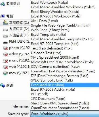
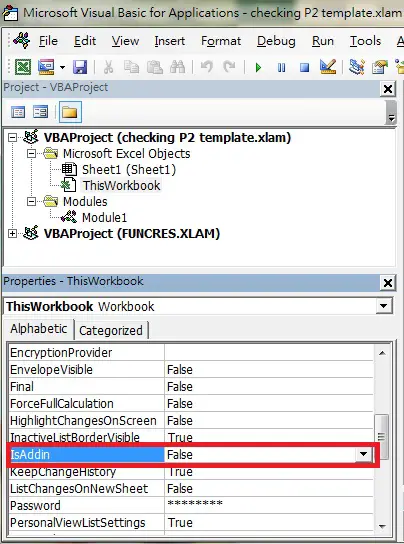
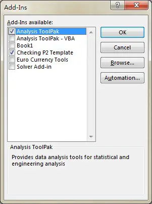
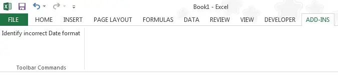
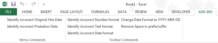
Create Excel Add-in and add in Ribbon

Excel Record Macro

Writing your first Excel Macro by recording Macro, why?

First of all, you should face the fact that you cannot know everything. You can use Microsoft Windows does not mean you can write your own Windows. Even if you are a Windows Administrator, it only means you have better knowledge on modifying parameters, but you do not need to how to write a Windows. Similarly, you can use Photoshop does not mean you can write the software. Depending on the role, different people are required different skill set, there are people who are “users”, some are “administrators”, and some are “developers”.

If you are a starter in Excel VBA, your role is changed from a “user” to a “developer”. It is a big change, you have to understand Excel well enough to make that change, and it takes a lot of efforts even if you are an expert user. During the transition, you should try being an “administrator”, someone who knows the software well and is able to modify parameters. Even as a developer, you don’t always need to write a program from zero, you just need to pull different sets of code together to become your own work.

As an administrator, you may not understand every line of code of a program but you should be able to change the parameters. Therefore, the first step of understanding Excel VBA is to record a Macro, read a program’s code and practice modifying the code and see what happens through trials and errors.

Understanding recorded Macro

Before continuing reading, you should have knowledge in recording Macro. Read the below article if you do not know how.

Excel Record Macro

Once you know the Excel VBA code behind an action, you can write your own actions or modify the code for your own need.

For example, you have recorded actions that do the followings

1) Select worksheet “Sheet1″

2) Type “1” in Range A1

3) Delete value in Range A1

Having recorded the above actions, go to VB Editor (Alt+F11) to see how the codes look like for each of those actions

1   Sub Macro1()
2      Sheets("Sheet1").Select
3      Range("A1").Select
4      ActiveCell.FormulaR1C1 = "1"
5      Range("A1").Select
6      Selection.ClearContents
7    End Sub

You can easily identify which line of code is representing the corresponding action. Now I am translating each code below into English.

1    Create a Macro called Macro1 with no parameters

2   Select worksheet “Sheet1″

3   Select Range A1

4   For the active cell (the one you have just selected), type formula  “1”

5   Select Range A1

6   For the selected Range, clear the contents

7   End of the Macro

It isn’t so hard to understand, right? Some codes are very easy to read, such as “Select”, “Range”, “Sheets”. If you don’t understand any of the code, just search it in goggle. For example, if you don’t understand what is FormulaR1C1, just search “Excel VBA FormulaR1C1″, and you will get a lot of results.

Writing your first Excel Macro

Now that you have identified the underlying code behind each action, you should be capable of writing your own first Excel Macro.

For example, I want to write “2” in A1 of “Sheet2″

1   Sub Macro2()      'change a different name for each Macro
 2      Sheets("Sheet2").Select
 3      Range("A1").Select
 4      ActiveCell.FormulaR1C1 = "2"
 5    End Sub

You have created your first VBA by modifying a recorded Macro, it is a good start! Try different actions like changing cell color, copy and paste, creating pivot table, search a text, and see how the codes look like, I assure you they are very easy and straight forward to use.

What’s Next?

There are things that cannot be recorded, but you should learn them step by step. The next thing you need to learn is the programming basics, such as define variables, VBA function, Objects and their Properties, condition (such as If..Else), Loop (such as For…Next)

You are recommended to read my other posts under the Excel VBA category in order of Unit.

Outbound References

https://www.youtube.com/watch?v=MYNVaRnZRgY

 

Writing your first Excel Macro by recording Macro

Excel verify Number data type and convert Text to Number

This Excel tutorial explains how to verify if a column contains only Number data type. If it is a Text then convert Text to Number.

Excel verify Number data type

Number can be in two forms in Excel – Text and Number. If a Number is a Text, there is a small triangle on the top left of the Cell.

By default, number in Text format aligns to the left while Number aligns to the right, but you can change the alignment.

There are three kinds of data in Excel – Date, Number and Text

To check whether the data is number, we have to make sure it is not Text and Date.

To make sure it is not a Text, Use IsNumer Function. IsNumber returns TRUE for Date and Number.

To make sure it is not  Date, use IsDate Function, Number is not considered as Date. Unfortunately, IsDate is for VBA only, we need to workaround with Cell Function for worksheet.

If the format is Date, Cell Function returns a value from D1 to D9, depending on the date format.

Now to combine IsNumber and Cell Function,

=IF(ISNUMBER(A2),IF(LEFT(CELL("Format",A2),1)="D",TRUE,FALSE))

Convert Text to Number

To convert Text to Number,select B2:B4, and then find the exclamation mark in B2, select “Convert to Number”.

Mass verification of Number data type (VBA)

Assume that you have hundreds of rows and columns with different required format, how should you check the data type?

First of all, create a row (row 1 in the example) that specifies the required data type for each column.

Now we can create a Macro that loops through row 1. If the required format is “Number”, then check  the data of the whole column whether it is a Text. The yellow Cells are in incorrect format that we want to identify in a new worksheet called “is not number”.

Public Sub isNotNumber()
On Error GoTo errHandler
    Set dataTypeRng = Application.InputBox("Input data Type Range", Type:=8)
    dataBeginRow = Application.InputBox("Input data begin row")
    dataEndRow = Application.InputBox("Input data end row")
    
    For Each Rng In dataTypeRng
        If Rng.Value = "Number" Then
            col_letter = Split(Rng.Address, "$")(1)
            For Each rng2 In Range(col_letter & dataBeginRow & ":" & col_letter & dataEndRow)
                If Not IsEmpty(rng2) And IsDate(rng2) Then
                    txt = txt & Replace(rng2.Address, "$", "") & " (Date)" & Chr(10)
                ElseIf Not IsEmpty(rng2) And Not Application.WorksheetFunction.IsNumber(rng2) Then
                    txt = txt & Replace(rng2.Address, "$", "") & " (Text)" & Chr(10)
                End If
            Next rng2
        End If
    Next Rng

    If txt <> "" Then
        For Each ws In ActiveWorkbook.Worksheets
            If Not wsExists("is not number") Then
                Set newWS = ThisWorkbook.Worksheets.Add
                newWS.Name = "is not number"
            End If
        Next ws
        Sheets("is not number").Select
        Sheets("is not number").Range("A1").Value = txt
    Else: MsgBox ("All Number format are correct")
   End If
    
errHandler: Exit Sub
End Sub

Function wsExists(wksName As String) As Boolean
    On Error Resume Next
    wsExists = CBool(Len(Worksheets(wksName).Name) > 0)
    On Error GoTo 0
End Function

Demonstration- Identify non-Number Cell

Run Macro

Type in the data Type Range

Type in the data being row

Type in the data end row

A worksheet called “is not number” is created, with the incorrect type inside the brackets. If you want to display them in A1, A2, A3… just copy the values to Notepad and then copy and paste back into Excel. I don’t want to create a Macro to correct the format because I think it is necessary to read Cell by Cell to understand what is causing the mistakes.

 

 

Excel verify Number data type and convert Text to Number

Excel VBA Msgbox and handling of return value

This Excel tutorial explains how to use Excel VBA Msgbox with carriage return such as vbCr, vbNewLine, and handling of return value such as vbOK, vbCancel, vbRetry

You may also want to read:

Excel VBA Inputbox and Application.Inputbox

What is Excel VBA MsgBox?

Excel VBA MsgBox is a prompt box that is used to prompt user for important information, usually provide user with OK and Cancel buttons. Note that there is another prompt box called InputBox which receives text input from user but it is not in the scope of this article.

Why do you need Excel VBA MsgBox?

There are several reasons that you may need Excel VBA Msgbox:

1) When you run a Sub or a Function, you will see the final result only and the result may not be what you expect while there is no error message. In that case, you can insert a Msgbox code within a Procedure to check the value of a variable at specific line of code.

2) To warn user or confirm an action, such as asking users if they confirm to delete data

Syntax of Excel VBA MsgBox

MsgBox(prompt[, buttons] [, title] [, helpfile, context])

Prompt	Required. String expression displayed as the message in the dialog box. The maximum length of Prompt is approximately 1024 characters, depending on the width of the characters used. If Prompt consists of more than one line, you can separate the lines using1) carriage return – Chr(13) or vbCr OR 2) line feed – Chr(10) or vbLf OR3) carriage return + line feed – Chr(13)& Chr(10) or vbCrLf  OR4) vbNewLine, suitable for different platforms
Buttons	Optional. Numeric expression that is the sum of values specifying the number and type of buttons to display, the icon style to use, the identity of the default button, and the modality of the message box. You can add more than one Buttons using + sign, such as vbOKCancel + vbExclamation If you omit Buttons, the default value is zero (The user must respond to the message box before continuing work in the current application.)If you choose a Button, you need to define a variable to return a value, otherwise you will receive the following error message. The return values are as follows Return Value Value vbOK 1 vbCancel 2 vbAbort 3 vbRetry 4 vbIgnore 5 vbYes 6 vbNo 7
Title	Optional. String expression displayed in the title bar of the dialog box. If you omit Title, the application name (Microsoft Excel) is placed in the title bar.
helpfile	Optional. String expression that identifies the Help file to use to provide context-sensitive Help for the dialog box. If helpfile is provided, context must also be provided.
context	Optional. Numeric expression that is the Help context number assigned to the appropriate Help topic by the Help author. If context is provided, helpfile must also be provided.

 

Buttons Argument (blue is about Modality)
Member	Value	Description
vbAbortRetryIgnore	2	Display Abort, Retry, and Ignore buttons.
vbApplicationModal	0	The user must respond to the message box before continuing work in the current application.
vbCritical	16	Display Critical Message icon.
vbDefaultButton1	0	First button is default.
vbDefaultButton2	256	Second button is default.
vbDefaultButton3	512	Third button is default.
vbDefaultButton4	768	Fourth button is default.
vbExclamation	48	Display Warning Message icon.
vbInformation	64	Display Information Message icon.
vbMsgBoxHelpButton	16384	Adds a Help button to the message box
vbMsgBoxRight	524288	Text is right aligned
vbMsgBoxRtlReading	1048576	Specifies text should appear as right-to-left reading on Hebrew and Arabic systems
vbMsgBoxSetForeground	65536	Specifies the message box window as the foreground window
vbOKCancel	1	Display OK and Cancel buttons.
vbOKOnly	0	Display OK button only (this is the default).
vbQuestion	32	Display Warning Query icon.
vbRetryCancel	5	Display Retry and Cancel buttons.
vbSystemModal	4096	System modal; all applications are suspended until the user responds to the message box
vbYesNo	4	Display Yes and No buttons.
vbYesNoCancel	3	Display Yes, No, and Cancel buttons.

Example of Excel VBA MsgBox

Step 1 – MsgBox with two lines of message

Public Sub test1()
    sInput = MsgBox("Are you sure to delete the data?" & vbNewLine & "Data will be deleted permanently")
End Sub

Step 2 – Add OK / Cancel Button

Public Sub test2()
    sInput = MsgBox("Are you sure to delete the data?" & vbNewLine & "Data will be deleted permanently", vbOKCancel)
End Sub

Step 3 – Add exclamation logo

 Public Sub test3()
    sInput = MsgBox("Are you sure to delete the data?" & vbNewLine & "Data will be deleted permanently", vbOKCancel + vbExclamation)
End Sub

Step 4 – Add message box title

Public Sub test4()
    sInput = MsgBox("Are you sure to delete the data?" & vbNewLine & "Data will be deleted permanently", vbOKCancel + vbExclamation, "Warning")
End Sub

Step 5 – Condition on return value

Public Sub test5()

sinput = MsgBox(“Are you sure to delete the data?” & vbNewLine & “Data will be deleted permanently”, vbOKCancel + vbExclamation, “Warning”)
    If sinput = vbOK Then
        ‘delete something
    ElseIf sinput = vbCancel Then
        ‘no action
    End If

End Sub

In the above example, we have OK and Cancel Buttons in MsgBox. If you click on the red cross on the top right, the return value is same as clicking on Cancel Button.

If your MsgBox contains only 1 button, clicking on the red cross is same as clicking on the only button, therefore red cross doesn’t necessarily mean Cancel.

 Outbound References

https://msdn.microsoft.com/en-us/library/office/gg251821%28v=office.15%29.aspx

Excel VBA Msgbox and handling of return value

Excel VBA Inputbox and Application.Inputbox

This Excel tutorial explains difference between VBA Inputbox and  Application.Inputbox and how to use them.

You may also want to read:

Excel VBA Msgbox and handling of return value

Excel VBA Inputbox and Application.Inputbox

Inputbox is pop up dialog box that displays a message and provides a text box for users to input free text. It is very similar to Msgbox except that Msgbox does not have a text box for user input.

There are two kinds of Inputbox: Inputbox and Application.Inputbox. Application.InputBox allows selective validation of the user’s input, and it can be used with Microsoft Excel objects, error values, and formulas. Note that Application.InputBox calls the InputBox method; InputBox with no object qualifier calls the InputBox function.

Syntax of Inputbox (Function)

InputBox(Prompt, [Title], [Default], [Left], [Top], [HelpFile], [HelpContextID])

Prompt	Required	The message to be displayed in the dialog box. If prompt consists of more than one line, you can separate the lines using a carriage return character (Chr(13)), a linefeed character (Chr(10)), or carriage return–linefeed character combination (Chr(13) & Chr(10)) between each line.
Title	Optional	The title for the input box. If this argument is omitted, the application name is placed in the title bar.
Default	Optional	String expression displayed in the text box as the default response if no other input is provided. If you omit default, the text box is displayed empty.
Left	Optional	Specifies an x position for the dialog box in relation to the upper-left corner of the screen, in points.If omitted, the dialog box is horizontally centered.
Top	Optional	Specifies a y position for the dialog box in relation to the upper-left corner of the screen, in points. If omitted, the dialog box is vertically positioned approximately one-third of the way down the screen.
HelpFile	Optional	The name of the Help file for this input box. If the HelpFile and HelpContextID arguments are present, a Help button will appear in the dialog box.
HelpContextID	Optional	The context ID number of the Help topic in HelpFile.

Example of Inputbox (Function)

The below example demonstrates how to create an input box for users to input their names, and then use the name in MsgBox.

Note that if user press Cancel button, use sinput = “” to capture.

 Public Sub inputFunction()
    sinput = InputBox("Please input your name", "User Input", "default value")
    If sinput = "" Then
        Exit Sub
    Else
        MsgBox ("Your name is " & sinput)
    End If
End Sub

 

When OK button is pressed

Syntax of Application.Inputbox (Method)

Application.InputBox(Prompt, [Title], [Default], [Left], [Top], [HelpFile], [HelpContextID], [Type])

Prompt	Required	The message to be displayed in the dialog box. If prompt consists of more than one line, you can separate the lines using a carriage return character (Chr(13)), a linefeed character (Chr(10)), or carriage return–linefeed character combination (Chr(13) & Chr(10)) between each line.
Title	Optional	The title for the input box. If this argument is omitted, the default title is “Input.”
Default	Optional	Specifies a value that will appear in the text box when the dialog box is initially displayed. If this argument is omitted, the text box is left empty. This value can be a Range object.
Left	Optional	Specifies an x position for the dialog box in relation to the upper-left corner of the screen, in points.If omitted, the dialog box is horizontally centered.
Top	Optional	Specifies a y position for the dialog box in relation to the upper-left corner of the screen, in points. If omitted, the dialog box is vertically positioned approximately one-third of the way down the screen.
HelpFile	Optional	The name of the Help file for this input box. If the HelpFile and HelpContextID arguments are present, a Help button will appear in the dialog box.
HelpContextID	Optional	The context ID number of the Help topic in HelpFile.
Type	Optional	Specifies the return data type. If this argument is omitted, the dialog box returns text. Value Description 0 A formula 1 A number 2 Text (a string) 4 A logical value (True or False) 8 A cell reference, as a Range object 16 An error value, such as #N/A 64 An array of values

As you can see, Application.Inputbox has one more argument “Type” which could perform validation.

Example of Application.Inputbox (Method)

The below example demonstrates how to create an input box for users to input their names, and then use the name in MsgBox.

You should use sinput = False to prevent error when users click on Cancel Button.

 Public Sub inputMethof()
    sinput = Application.InputBox("Please input your name", "User Input", "default value")
    If sinput = False Then
        Exit Sub
    Else
        MsgBox ("Your name is " & sinput)
    End If
End Sub

You may set the Range using Type:=8 in the last argument. In this case, you should use On Error to prevent error from pressing Cancel Button as well as setting value as Range.

Public Sub inputRanged()
On Error GoTo errHandler:
    Set rng = Application.InputBox("Please input data Range", "User Input", Type:=8)
    rng.Interior.ColorIndex = 19
errHandler: Exit Sub
End Sub

If you enter a value that is not correct (not a Range), an error message will pop up and then return you to the Inputbox. This is how the validation of data type is done with Application.Inputbox, such checking applies to other formats as well.

If you does not like the message from validation to pop up, turn it off with

Application.DisplayAlerts = False

Outbound References

https://msdn.microsoft.com/en-us/library/office/ff839468.aspx

https://msdn.microsoft.com/en-us/library/office/gg251811.aspx

Excel VBA Inputbox and Application.Inputbox

Create Excel Add-in and add in Ribbon

This Excel tutorial explains how to add Excel Add-in in Ribbon.

Why use Excel Add-in

After you have created a Macro (Sub Procedure), you may want to distribute it for users to use. You can simply add the VBA code in the Module of a Workbook and then distribute the Workbook, but the problem is that the Macro cannot be used in other Workbook.

Depending on the situation, you may want to distribute a Macro is through Add-in. Add-in is a file with extension .xla (for Excel 2003 and older version) and .xlam (for Excel 2007 and newer version) where users can use the Macro in any Workbook in his workstation. The Add-in itself is stored in the local drive of the receiver, it is not stored in a Workbook. If you have used Functions from Analysis ToolPak before, you realize that if you send the Workbook that used the Function (such as MRound, Networkdays) to others who do not have the Add-in, the formula will fail once refreshed.

To summarize, if your Macro is only for use in particular Workbook, you don’t have to use Add-in. If not, create an Add-in.

After creating an Excel Add-in, send the Add-in to users, then install the add-in.

In order to facilitate users to locate and run the Macro, I highly recommend to add the Macro in Ribbon.

In the following demonstration, I will use a real example where I create several Macro for users to validate data, such as data formatting and conflicting values.

Create Excel Add-in

Assume that you have already created several Sub Procedure in the Module of a Workbook. The next step is to tell Excel to create a ribbon.

In VBE (Alt+F11), double click on ThisWorkBook under VBA Project of the Add-In, we need to add two Events here:

Workbook.AddinInstall Event – Triggered when users install the Add-in. We are going to tell Excel to add ribbon here.

Workbook.AddinUninstall Event – Triggered when users uninstall the Add-in. We are going to tell Excel to remove ribbon here.

Insert the following code in ThisWorkbook

Private Sub Workbook_AddinInstall()
    With Application.CommandBars("Formatting").Controls.Add
        .Caption = "Identify incorrect Date format" 'The button caption
        .Style = msoButtonCaption
        .OnAction = "checkDateText" 'The Macro name you want to trigger
    End With
End Sub

Private Sub Workbook_AddinUninstall()
 On Error Resume Next
    Application.CommandBars("Formatting").Controls("Identify incorrect Date format").Delete
 On Error GoTo 0
End Sub

The above code adds a button called Identify incorrect Date format. If you want to add more, copy the code and change the Caption and OnAction parameters.

Save Excel Add-In

Save the Workbook as you would normally save it, except that you save it as xlam file type for Add-In. Name the file as checking P2 template.

The xlam file icon looks like Excel, you can send this file for users to install.

After you have saved the file as .xlam, all worksheets are hidden.

To change it back to a normal worksheet, change the IsAddin Property of ThisWorkbook to False.

Install Excel Add-in (User)

Navigate to Developer tab > Add-Ins, browse the Add-In location to add.

Now a tab called ADD-INS is added, under which is the button “Identify incorrect Date format”

If you have many items, you can group items by different CommandBars as below.

In the above example, I grouped them by Formatting / Worksheet Menu Bar

    With Application.CommandBars("Formatting").Controls.Add
        .Caption = "Remove Space in prefix/suffix"
        .Style = msoButtonCaption
        .OnAction = "checkSpace"
    End With 
        
    With Application.CommandBars("Worksheet Menu Bar").Controls.Add
        .Caption = "Identify incorrect Original Hire Date"
        .Style = msoButtonCaption
        .OnAction = "chk_Original_Hire_Dt"
    End With

http://sitestory.dk/excel_vba/my_menu.htm

Create Excel Add-in and add in Ribbon

Excel PERCENTILE.INC vs PERCENTILE.EXC

This Excel tutorial explains how to use Percentile related Functions, include PERCENTILE, PERCENTILE.INC, PERCENTILE.EXC.

Excel Percentile

Percentile is a statistics term used to describe the Nth observation in a data set after sorting in ascending order. For example, 40th percentile (P40) refers to the approximately 40th data of the 100 data. If the data set is not exactly 100, say 200, we find the location of observation at 40% of total data.

Percentile is commonly used in salary survey to find out the 25th 50th, 75th, 90th percentile. 50% percentile is known as median, human resources department always compares P50 salary with employees’ salary so that they know who are below market compensation. Some companies may have salary guideline of P75, which means they generally pay better than the market in order to attract and retain talents. Percentile is a better measure than average because extreme data are disregarded using percentile.

There are three Functions to calculate percentile in Excel (PERCENTILE, PERCENTILE.INC, PERCENTILE.EXC). Before we look into the difference, let’s look at an example of manual calculation.

Percentile – Manual calculation

There are basically two kinds of percentile calculation. Although the results are slightly different, both are considered correct. If you want to know all other methods, click here.

Method 1 – using (n+1)*p

This is the most common approach written in college statistics text book.

To calculate percentile, find out the location (or rank) of the percentile first

Location of a Percentile  = (total number of observations + 1) * (target percentile / 100)

Using the data set 1, 3, 5, 7 as example,

Location of P75 = (4+1)*(75/100)

============== 3.75

The 3.75th percentile is three quarters of the distance between the third and forth observation, therefore

Value of P75 = 3rd observation + (4th observation -3rd observation ) * 0.75

=========== 5+(7-5)*0.75

=========== 6.5

Method 2 – using (n-1)*p+1

Method 1 and Method 2 are only different when the calculated location (rank) of percentile is non-integer.

Location of a Percentile  = (total number of observations - 1) * (target percentile / 100) + 1

Using the data set 1, 3, 5, 7 as example,

Location of P75 = (4-1)*(75/100)+1

============== 3.25

Value of P75 = 3rd observation + (4th observation -3rd observation ) * 0.25

=========== 5+(7-5)*0.25

=========== 5.5

Percentile – Excel calculation

There are three Functions relating to percentile in Excel :PERCENTILE, PERCENTILE.INC, PERCENTILE.EXC

If you want to calculate percentile using Method 1, use PERCENTILE.EXC Function.

If you want to calculate percentile using Method 2, use PERCENTILE or PERCENTILE.INC Function, both are the same.

PERCENTILE.EXC and PERCENTILE.INC are new versions of PERCENTILE. PERCENTILE remains in Excel for compatibility purpose only, you can ignore this Function.

Syntax

All three Functions have the same arguments

PERCENTILE(array, k)

PERCENTILE.INC(array, k)

PERCENTILE.EXC(array, k)

array	The array or range of data that defines relative standing.
k	The percentile value in decimal number

PERCENTILE.EXC works if k is between 1/n and 1-1/n, while PERCENTILE.INC works if k is between 0 and 1.

Example

Suppose data set 1, 3, 5, 7 lie in Range A1:A4. To find P75

Method 1:

= PERCENTILE.EXC(A1:A4,0.75)

= 6.5

Method 2:

= PERCENTILE.INC(A1:A4,0.75)

= 5.5

 

Excel PERCENTILE.INC vs PERCENTILE.EXC

Excel central tendency (mean mode median)

This Excel tutorial explains how to use mean, mode and median to measure Central Tendency.

Excel Central Tendency

Central Tendency is a statistics term to describe the central point of probability distribution. Central Tendency can be measured by mean, mode and median. This tutorial explains how to use Excel to measure mean, mode and median using Excel formula.

Arithmetic Mean

Definition

Arithmetic Mean is also known as mean or average. Simply speaking, it is sum of all numbers and then divide by how many numbers that you have summed.

There are two kinds of mean in statistics – population mean and sample mean, represented by the following notations.

  =  population mean

  =  sample mean

Population mean is to average all numbers, while sample mean is to average part of the population. For example, we want to study if U.S. citizens like Obama, apparently we cannot ask everyone in the U.S., instead we just ask some of the people (sample) and then use the result to estimate how all the U.S. citizens (population) think.

Excel

In Excel, use the Function Average to calculate mean.

For example, from cell A1 to A6, we have the following data set.

1
2
3
4
5
6

The mean of these numbers =AVERAGE(A1:F1)

The result is 3.5

If you try to apply filter and then calculate average value, use Subtotal Function to do that.

Median

Definition

Place all the observations in order (ascending or descending) and find the data in the middle point.

If the number of observations is odd number, we can easily find the middle point. In the below example, 3 is the median.

1
2
3
4
5

If the number of observations is even number, sum up the two values closest to the middle point and then divide by 2.

In the below example, median = (3+4)/2 = 3.5

1
2
3
4
5
6

Most of the surveys use Median instead of Average, for example, household income. The reason is that we want to avoid extreme cases such as Bill Gates’s income, which would shift the average income higher than our expectation (See the below right skew diagram). Therefore median is a better measurement of central tendency for this case.

Excel

Given a data set from Range A1 to A6 as below

1
2
3
4
5
6

Apply formula  =Median(A1:A6)

The result is 3.

Note that you don’t have to sort the data yourself before you apply Median, just select the range of data.

Mode

Definition

Mode is the most frequently occurring value in the data set.

Excel

In Excel, use Mode Function to find Mode.

For example, from cell A1 to A6, we have the following data set.

Apply formula  =Mode(A1:F1)

The result is 1

Outbound References

https://statistics.laerd.com/statistical-guides/measures-central-tendency-mean-mode-median.php

 

Excel central tendency (mean mode median)

1

1

1

2

2

3

Excel Display Time from Date Time

This Excel tutorial explains how to use Custom Format to display Time from Date Time.

You may also want to read:

Excel Extract Time from Date Time

Excel Custom Format

Excel Display Time from Date Time

In my previous post, I have explained how to extract time from date time. What I mean “extract” is that the date is using formula to  completely remove date from date time. In this tutorial, I will explain how to use custom format to display Date Time in Time format.

Custom Format to display Time

To change how Date Time is displayed, right click on the Cell containing the Date Time > Format Cells > Custom

Below are some Custom Formats for time.

hh	Express hour from 01 to 24. If hour exceeds 24, a day will add and hour will be subtracted by 24
mm	Express month in number, from 01 to 12
ss	Express second from 01 to 59. If second exceeds 60, a minute will add and second will be subtracted by 60
[hh]	Convert date and time to hours, allow you to display hour larager than 24
[mm]	Convert date and time to minute, allow you to display minute larger than 60
[ss]	Convert date and time to second allow you to display second larger than 60

If you want to completely ignore the Date from Date Time, format the Cell as hh:mm

For example,  1/1/2014  1:01:01 is displayed as 01:01

If you want to display hh:mm but you want to convert Date (24 hour for 1 day) to hh, use [hh]:mm

For example, 1/1/2014  1:01:01 is displayed as 999361:01

99361 is the number of hours past since 1/1/1900 00:00:00

Similarly, you can use [mm] to convert Date+Hour to minute, use [ss] to add Date+Hour+Minute to second.

If you want to use formula to do conversion instead of simply changing the display, you can use the Text formula. For example,

=TEXT(D2,”[hh]:mm”)

Outbound References

https://support.office.com/en-us/article/Create-a-custom-number-format-78f2a361-936b-4c03-8772-09fab54be7f4?CorrelationId=f9dfc98c-1186-44d5-b23c-5843840ad1ec&ui=en-US&rs=en-US&ad=US

 

Excel Display Time from Date Time

Excel clustered column chart

This Excel tutorial explains how to use clustered column chart to compare a group of bar charts.

Excel clustered column chart

Clustered column chart is very similar to bar chart, except that clustered column chart allow grouping of bars for side by side comparison. This tutorial demonstrates how to build clustered column chart.

Example – clustered column chart

Suppose we want to build a sales bar chart for Q1 to Q4 in 2015. We can simply build a bar chart that shows sales of each quarter in each bar. But what if we also want to compare the sales in 2014 for each quarter (year over year comparison) ?

Now create a matrix as below

In Excel 2013, select data from A1 to C5, > Insert > Insert Column Chart > More Column Charts

Under Clustered Column, there are two options as below. One is x-axis grouped by year, and the other is grouped by quarter.

In this example, we want to compare each quarter side by side, so we choose the first option.

Modify clustered column chart

Although we have completed the graph, we also want to know how to modify the graph parameter.

Now right click on the graph and click on Select Data

On the right hand side Horizontal Axis Labels, we can modify the X axis Labels by clicking on Edit button. In our example, we select Range A2:A5 in order to show Q1 sales to Q4 sales labels.

On the left hand side Legend Entries,  2014 and 2015 represent the y axis value of the bars, they are two sets of data so we need to add two entries (2014 and 2015) if we manually select the data.

Assume that we have 2016 data in column D and we want to add it to the existing graph.

Click on Add button, and then fill in the Edit Series box as below.

Format clustered column chart

Most formatting are self explanatory, but one notable option is Series Overlap, you can adjust it to prevent the gap between each bar within the same group.

Outbound References

http://www.ehow.com/how_8500994_create-clustered-stacked-chart-excel.html

 

 

Excel clustered column chart

Access Excel add leading zero

This Access / Excel tutorial explains how to add leading zero using Text Function or using custom Function to pad other text in suffix or prefix.

Excel add leading zero

Number in Excel can come in two forms – Text or Number.

For number in Number format, you may not add zero in prefix

For number in Text format, you can add a zero in prefix

In order to convert a Number to Text, add a ‘ in the prefix. For example, instead of typing 00123, type ‘00123

Sometimes you receive data originally in Text format such as 00123 but the formatting is lost and it becomes Number format 123. Assume that you know how many digits the text originally has, say 8 digits, then you can make use of Text Function.

=Text(A1, “00000000”)

Now you can see the leading zero makes up to 8 digits.

Access Excel VBA custom Function to add text in prefix or suffix

I created two custom Functions to simulate Oracle PL/SQL Functions LPad (left pad) and RPad (right pad), which are used to add any text in prefix or suffix up to specific number of characters.

This custom Function can be used in Access and Excel.

Left Pad (add leading zero in prefix)

Syntax

wLpad(sInput, digits, padString)

sInput	The text to be manipulated
digits	Number of characters to add in prefix
padString	The text to be added to sInput, must be one character

VBA Code

Public Function wLpad(sInput As String, digits As Integer, padString As String) As String
    sInputLen = Len(sInput)
    If digits <= sInputLen Then
        result = sInput
    Else
        For i = 1 To (digits - sInputLen)
            result = result & padString
        Next i
        result = result & sInput
    End If
    wLpad = result
End Function

Example

Number	Formula	Result
1	=wLpad(A2,8,0)	00000001
12	=wLpad(A3,8,0)	00000012
123	=wLpad(A4,8,0)	00000123
1234	=wLpad(A5,8,0)	00001234
12345	=wLpad(A6,8,0)	00012345
123456	=wLpad(A7,8,0)	00123456
1234567	=wLpad(A8,8,0)	01234567
12345678	=wLpad(A9,8,0)	12345678
123456789	=wLpad(A10,8,0)	123456789

Right Pad (add zero in suffix)

Syntax

wRpad(sInput, digits, padString)

sInput	The text to be manipulated
digits	Number of characters to add in suffix
padString	The text to be added to sInput, must be one character

VBA Code

Public Function wRpad(sInput As String, digits As Integer, padString As String) As String
    sInputLen = Len(sInput)
    If digits <= sInputLen Then
        result = sInput
    Else
        For i = 1 To (digits - sInputLen)
            result = result & padString
        Next i
        result = sInput & result
    End If
    wRpad = result
End Function

Example

Number	Formula	Result
1	=wRpad(A2,8,0)	10000000
12	=wRpad(A3,8,0)	12000000
123	=wRpad(A4,8,0)	12300000
1234	=wRpad(A5,8,0)	12340000
12345	=wRpad(A6,8,0)	12345000
123456	=wRpad(A7,8,0)	12345600
1234567	=wRpad(A8,8,0)	12345670
12345678	=wRpad(A9,8,0)	12345678
123456789	=wRpad(A10,8,0)	123456789

 

 

Access Excel add leading zero

Excel loop workbooks in folders and subfolders with FSO

This Excel tutorial explains how to loop workbooks in folders and subfolders with FileSystemObject (FSO).

Excel loop workbooks in folders and subfolders

FileSystemObject (FSO) provides an API to access the Windows filesystem such as accessing Drive, TextStram, Folder, File. In this tutorial, since we are discussing how to loop workbook in folders and subfolders, I will only explain the use of Folder and File.

FSO can also be used in other Microsoft Products such as ASP, Word, Access, etc. Therefore you just need to modify the workbook specific Objects in my examples in order to use the code in other products.

You should be able to run FSO in Excel 2013. If you fail to run FSO Object, open VBE (ALT+F11) > Tools > References > Check the box Microsoft Scripting Runtine

After using FSO, you can loop workbooks in a folder and do whatever you want. In this tutorial, I will show some examples which you can copy and modify at ease.

Modify workbooks in folders and subfolders

The below Procedure open and close the workbooks in the folders and subfolders, you can further add your own code to modify the workbooks.

Public Sub openWB()
    Dim FSO As Object
    Dim folder As Object, subfolder As Object
    Dim wb As Object
    
    Set FSO = CreateObject("Scripting.FileSystemObject")
    folderPath = "C:\Users\WYMAN\Desktop\testDel"
    Set folder = FSO.GetFolder(folderPath)
    
    With Application
        .DisplayAlerts = False
        .ScreenUpdating = False
        .EnableEvents = False
        .AskToUpdateLinks = False
    End With
        
    For Each wb In folder.Files
        If Right(wb.Name, 3) = "xls" Or Right(wb.Name, 4) = "xlsx" Or Right(wb.Name, 4) = "xlsm" Then
            Set masterWB = Workbooks.Open(wb)
  'Modify your workbook
            ActiveWorkbook.Close True
        End If
    Next
    For Each subfolder In folder.SubFolders
        For Each wb In subfolder.Files
            If Right(wb.Name, 3) = "xls" Or Right(wb.Name, 4) = "xlsx" Or Right(wb.Name, 4) = "xlsm" Then
                Set masterWB = Workbooks.Open(wb)
 'Modify your workbook
                ActiveWorkbook.Close True
            End If
        Next
    Next
    With Application
        .DisplayAlerts = True
        .ScreenUpdating = True
        .EnableEvents = True
        .AskToUpdateLinks = True
    End With
End Sub

Delete workbook in folder and subfolder

The below Procedure deletes workbooks in a folder and its subfolders.

Public Sub delWB()
    Dim FSO As Object
    Dim folder As Object, subfolder As Object
    Dim wb As Object
    
    Set FSO = CreateObject("Scripting.FileSystemObject")
    folderPath = "C:\Users\WYMAN\Desktop\testDel"
    Set folder = FSO.GetFolder(folderPath)
    
    For Each wb In folder.Files
        If Right(wb.Name, 3) = "xls" Or Right(wb.Name, 4) = "xlsx" Or Right(wb.Name, 4) = "xlsm" Then
           FSO.DeleteFile wb, True
        End If
    Next
    For Each subfolder In folder.SubFolders
        For Each wb In subfolder.Files
            If Right(wb.Name, 3) = "xls" Or Right(wb.Name, 4) = "xlsx" Or Right(wb.Name, 4) = "xlsm" Then
                FSO.DeleteFile wb, True
             End If
        Next
    Next
End Sub

Other related FSO Methods

Now that you have understood the basics to loop workbooks, but you may also want to move around the folders or files, click the below articles to read more.

FSO File Methods

FSO Folder Methods

Further Workbook actions you may want to do

After you have looped through workbooks, you may want to do the followings

Auto run Macro when workbook is opened

Consolidate worksheets into one worksheet

Extract columns with specific header to new workbook

Find all external links and broken links in workbook

Loop through all worksheets in the same workbook

Refresh closed workbook (links / Pivot Tables)

 Outbound References

https://msdn.microsoft.com/en-us/library/7kby5ae3%28v=vs.84%29.aspx

Excel loop workbooks in folders and subfolders with FSO

Access Excel FSO File Methods

This Access / Excel tutorial explains how to use FSO File related Methods including FileExists, DeleteFile, MoveFile, CopyFile

You may also want to read:

Access Excel FSO Folder Methods

FSO File Methods

FileSystemObject (FSO) provides an API to access the Windows filesystem such as accessing Drive, TextStram, Folder, File. In this tutorial, I will only explain the use of some important File related Methods. For details, please read the MSDN library.

You should be able to run FSO in Excel 2013. If you fail to run FSO Object, open VBE (ALT+F11) > Tools > References > Check the box Microsoft Scripting Runtine

FileExists Method

Check if a file already exists in the directory, returning True or False. See the below example.

DeleteFile Method

DeleteFile Method deletes a File, returns an error if File does not exist.

Syntax

object.DeleteFile filespec[, force]

object	Required. Always the name of a FileSystemObject.
filespec	Required. The name of the file to delete. The filespec can contain wildcard characters in the last path component.
force	Optional. Boolean value that is True if files with the read-only attribute set are to be deleted; False (default) if they are not.

Example

The below Procedures deletes a file if it already exists.

Public Sub delFile()
    Set FSO = CreateObject("Scripting.FileSystemObject")
    If FSO.FileExists("C:\Users\WYMAN\Desktop\testDel.xlsx") = True Then
        FSO.deleteFile ("C:\Users\WYMAN\Desktop\testDel.xlsx")
    End If
End Sub

MoveFile Method

MoveFile Method moves a file to another location. Error occurs if source or destination path cannot be found.

Syntax

object.MoveFile source, destination

object	Required. Always the name of a FileSystemObject.
source	Required. The path to the file or files to be moved. The source argument string can contain wildcard characters in the last path component only.
destination	Required. The path where the file or files are to be moved. The destination argument can’t contain wildcard characters.

Example

The below Procedures move a file from Desktop to C:\test\, overwriting existing file in destination.

Public Sub movFile()
    movFromPath = "C:\Users\WYMAN\Desktop\testDel.xlsx"
    movToPath = "C:\test\testDel.xlsx"
   
    Set FSO = CreateObject("Scripting.FileSystemObject")
    If FSO.FileExists(movFromPath) = True Then
        If FSO.FileExists(movToPath) = False Then
           FSO.movefile movFromPath, movToPath
        Else
           FSO.deleteFile movToPath
           FSO.movefile movFromPath, movToPath
        End If
    End If
End Sub

CopyFile Method

Copy a File to another location. If the File already exists in destination, an error occurs.

Syntax

object.CopyFile source, destination[, overwrite]

object	Required. Always the name of a FileSystemObject.
source	Required. Character string file specification, which can include wildcard characters, for one or more files to be copied.
destination	Required. Character string destination where the file or files from source are to be copied. Wildcard characters are not allowed.
overwrite	Optional. Boolean value that indicates if existing files are to be overwritten. If True, files are overwritten; if False, they are not. The default is True. Note that CopyFile will fail if destination has the read-only attribute set, regardless of the value of overwrite.

Example

The below Procedures copy a File from Desktop to C:\test\, overwriting existing File.

Public Sub cpyFile()
    copyFromPath = "C:\Users\WYMAN\Desktop\testDel.xlsx"
    copyToPath = "C:\test\testDel.xlsx"
   
    Set FSO = CreateObject("Scripting.FileSystemObject")
    If FSO.FileExists(copyFromPath) = True Then
        FSO.copyfile copyFromPath, copyToPath, True
    End If
End Sub

Other File related Methods

Below are some less commonly used Methods related to File, click on the hyperlink to read the details.

GetFile	Returns a File object corresponding to the file in a specified path.
GetFileName	Returns the last component of specified path that is not part of the drive specification.

 

Access Excel FSO File Methods

Access Excel FSO Folder Methods

This Access / Excel tutorial explains how to use FSO Folder related Methods including FolderExists, CreateFolder, DeleteFolder, MoveFolder, CopyFolder

FSO Folder Methods

FileSystemObject (FSO) provides an API to access the Windows filesystem such as accessing Drive, TextStram, Folder, File. In this tutorial, I will only explain the use of some important Folder related Methods. For details, please read the MSDN library.

You should be able to run FSO in Excel 2013. If you fail to run FSO Object, open VBE (ALT+F11) > Tools > References > Check the box Microsoft Scripting Runtine

FolderExists Method

Check if a folder already exists in the directory, returning True or False. See the below example.

CreateFolder Method

CreateFolder Method creates a Folder, it returns an error if Folder already exists.

Syntax

object.CreateFolder(foldername)

object	Required. Always the name of a FileSystemObject.
foldername	Required. String expression that identifies the folder to create.

Example

The below Procedures create a folder if not exists.

Public Sub mkFolder()
    Set FSO = CreateObject("Scripting.FileSystemObject")
    If FSO.FolderExists("C:\Users\WYMAN\Desktop\testDel") = False Then
        FSO.createFolder ("C:\Users\WYMAN\Desktop\testDel")
    End If
End Sub

DeleteFolder Method

DeleteFolder Method deletes a Folder regardless whether it has contents inside. The method returns an error if Folder does not exist.

Syntax

object.DeleteFolder folderspec[, force]

object	Required. Always the name of a FileSystemObject.
folderspec	Required. The name of the folder to delete. The folderspec can contain wildcard characters in the last path component.
force	Optional. Boolean value that is True if folders with the read-only attribute set are to be deleted; False (default) if they are not.

Example

The below Procedures deletes a folder if it already exists.

Public Sub delFolder()
    Set FSO = CreateObject("Scripting.FileSystemObject")
    If FSO.FolderExists("C:\Users\WYMAN\Desktop\testDel") = True Then
        FSO.deleteFolder ("C:\Users\WYMAN\Desktop\testDel")
    End If
End Sub

MoveFolder Method

MoveFolder Method moves a folder to another location. Error occurs if source or destination cannot be found.

Syntax

object.MoveFolder ( source, destination );

object	Required. Always the name of a FileSystemObject.
source	Required. The path to the folder or folders to be moved. The source argument string can contain wildcard characters in the last path component only.
destination	Required. The path where the folder or folders are to be moved. The destination argument can’t contain wildcard characters.

Example

The below Procedures move a folder from Desktop to C:\, overwriting existing folder in destination.

Public Sub movFolder()
    copyFromPath = "C:\Users\WYMAN\Desktop\testDel"
    copyToPath = "C:\testDel"
   
    Set FSO = CreateObject("Scripting.FileSystemObject")
    If FSO.FolderExists(copyFromPath) = True Then
        If FSO.FolderExists(copyToPath) = False Then
           FSO.movefolder copyFromPath, copyToPath
        Else
           FSO.deleteFolder copyToPath
           FSO.movefolder copyFromPath, copyToPath
        End If
    End If
End Sub

CopyFolder Method

Copy a Folder to another location. If the Folder already exists in destination, an error occurs.

Syntax

object.CopyFolder ( source, destination[, overwrite] )

object	Required. Always the name of a FileSystemObject.
source	Required. Character string folder specification, which can include wildcard characters, for one or more folders to be copied.
destination	Required. Character string destination where the folder and subfolders from source are to be copied. Wildcard characters are not allowed.
overwrite	Optional. Boolean value that indicates if existing folders are to be overwritten. If true, files are overwritten; if false, they are not. The default is true.

Example

The below Procedures copy a folder from Desktop to C:\, overwriting existing Folder.

I tested the overwrite argument but it fails to overwrite an existing folder, so I delete the folder instead.

Public Sub cpyFolder()
    copyFromPath = "C:\Users\WYMAN\Desktop\testDel"
    copyToPath = "C:\testDel"
   
    Set FSO = CreateObject("Scripting.FileSystemObject")
    If FSO.FolderExists(copyFromPath) = True Then
        If FSO.FolderExists(copyToPath) = False Then
           FSO.copyfolder copyFromPath, copyToPath
        Else
           FSO.deleteFolder copyToPath
           FSO.copyfolder copyFromPath, copyToPath
        End If
    End If
End Sub

Other Folder related Methods

Below are some less commonly used Methods related to Folder, click on the hyperlink to read the details.

GetFolder	Returns a Folder object corresponding to the folder in a specified path.
GetParentFolderName	Returns a string containing the name of the parent folder of the last component in a specified path.
GetSpecialFolder	Returns the special folder object specified.

 

Access Excel FSO Folder Methods

Access create Relationships

This Access tutorial explains how to create Relationships and the purpose of Enforce Referential Integrity.

You may also want to read:

Access Table add subdatasheet

Access create Relationships

Create Relationships in Access is about telling Access how one table relates to another table. This process is not mandatory, you can still do everything without building any Relationships. However, if you are going to build an application, it can help you make sure all related tables are updated at the same time.

Assume that we have two tables – Compensation and Job. When an employee is hired, an Employee ID is created in Job, therefore it contains all Employee ID. Afterward a compensation record is created.

Compensation

Employee ID	Salary	Allowance
1	10000	100
2	20000	200
3	30000	300
4	40000	400
5	50000	500
6	60000	600

 

Job

Department	Employee ID	Employment Date
Account	1	1/1/2000
Admin	2	1/1/2001
Admin	3	1/1/2002
Admin	4	1/1/2003
Payroll	5	1/1/2004
HR	6	1/1/2005
Finance	7	1/1/2006

In Access 20013, click on DATABASE TOOLS tab >Relationships

You will see there are three Tables inside. These are default Relationships, you can ignore them.

Drag the Job and Compensation tables from Navigation Pane to Relationships.

Highlight Employee ID in Job, hold down mouse button and drag over to Employee ID in Compensation.

It is important that you drag from Job to Compensation but not the other way round. The table you drag from (Job) is the master table storing the Employee ID, any changes you make to Employee ID is made in this table first. The table you drag to (Compensation) is the table being affected by the change of master table.

Now the below menu pops up.

Relationship Type

At the bottom, the Relationship Type reflects whether the selected fields are Primary Key.

One to One – Both Employee ID are Primary Key (you must enable Enforce Referential Integrity to see the number 1 on the line)

One to Many – Only one of the Employee ID is Primary Key (you must enable Enforce Referential Integrity to see the number 1 and many symbol on the line)

Indeterminate (Many to Many) – Both Employee ID are not Primary Key

Data Integrity

Above Relationship Type, there are three options relating to data Integrity.

You must add at least one of the Employee ID as Primary Key in order to enable Enforce Referential Integrity and its sub options. (Not allow Many to Many relationship)

Enforce Referential Integrity (add data)

This option prevents users to add a new Employee ID in Compensation where the new Employee ID does not exist in Job.

Cascade Update Related Fields (update data)

When checked, whenever you update Employee ID in Job, Employee ID in Compensation also changes.

Cascade Delete Related Fields (delete data)

When checked, whenever you delete Employee ID in Job, records containing that Employee ID in Compensation also get deleted.

Effect of Relationships on Subdatasheet

In the Design View of Job table, the property Subdatasheet Name is [Auto] by default.

After adding the Relationships, you can see the linked Compensation data in Job table Datasheet View.

If you don’t like it, you can change the Subdatasheet Name property to [None].

Outbound References

https://msdn.microsoft.com/en-us/library/office/ff191810.aspx

Access create Relationships