2015年4月20日 星期一

Excel VBA Application Volatile Method to force recalculate

This Excel tutorial explains the use of Application Volatile Method to recalculate custom Function (User Defined Function).


You may also want to read:


Excel Workbook Calculation Automatic and Manual


Excel VBA Application Volatile Method


In Excel VBA, you can create your own Functions, we call it User Defined Function (UDF), usually I simply call it custom Function. Function is a Procedure that can take argument and return a value.


There are two kinds of custom Functions.


The first kind does not need to reference to other Cells, the Function can have an argument with constant value or without an argument. For example, you can use Rnd Function inside a custom Function to generate a number, therefore you don’t need any reference.


The second kind needs to reference to other Cells and return a value. For example, you need to reference to a Range when you use SUM Function.


Excel uses a special mechanism to minimize the number of calculation to speed up the process.  Excel builds “Dependency Trees”, which keeps track on the following changes


  • Formulae/Names that have changed.

  • Formulae containing Volatile Functions

  • Formulae dependent on changed or volatile formulae or cells or names

Navigate to Excel Options to turn Workbook Calculation to Automatic,  then your formula Cell will recalculate automatically if the relationship is in the Dependency Trees.


workbook_calculation_01


According to the above rules, Functions that do not depend on other changed cells would not recalculate, unless Application Volatile Method is used.


To illustrate the above concepts, I refer to the custom Functions I previously wrote.


Custom Function that do no require Application Volatile Method


In the previous post, I wrote a custom Function to count substring in a string, for example, it can count how many “p” appears in “apple”.


Public Function wCountSubStr(str As String, substr As String) As Integer
    lenstr = Len(str)
    lensubstr = Len(substr)
    
    For i = 1 To lenstr
        tempString = Mid(str, i, lensubstr)
        If tempString = substr Then
            count = count + 1
        End If
    Next i
    wCountSubStr = count
End Function

This Function requires two parameters, if you refer the argument to a Cell, the Function would recalculate automatically when the Cell changes.


For example,  the formula recalculates every time A1 value is changed.


=wCountSubStr(A1,”p”)


Custom Function that requires Application Volatile Method


In the below example, the Function does not have any argument and the result depends on A1.


Function test()
    test = Range("A1").Value * 2
End Function

Excel cannot recognize you are referencing A1 value because Excel builds the Dependency Tree using reference in arguments but not VBA. So even if you change A1, the formula would not recalculate automatically.


If you insert Application Volatile Method in this Function, this Function will recalculate whenever a Cell is edited, regardless of whether it is Cell A1 or not, therefore Application Volatile should be avoided if possible as it slows down Excel performance.


Function test()
   Application.Volatile
    test = Range("A1").Value * 2
End Function

Outbound References


https://msdn.microsoft.com/en-us/library/office/ff195441.aspx


Excel VBA Application Volatile Method to force recalculate

Excel Range Sort Method to sort data

This Excel tutorial explains how to sort Excel data using Excel VBA Sort Method, and how to sort dynamic Range.


You may also want to read


Excel Table AutoFilter sorting


Excel Worksheet AutoFilter sorting


Excel Range Sort Method to sort data


There are mainly three kinds of sorting in Excel.


1 – Table AutoFilter sorting, using List Object to access AutoFilter.


2 – Worksheet Autofilter sorting, using Range to access AutoFilter.


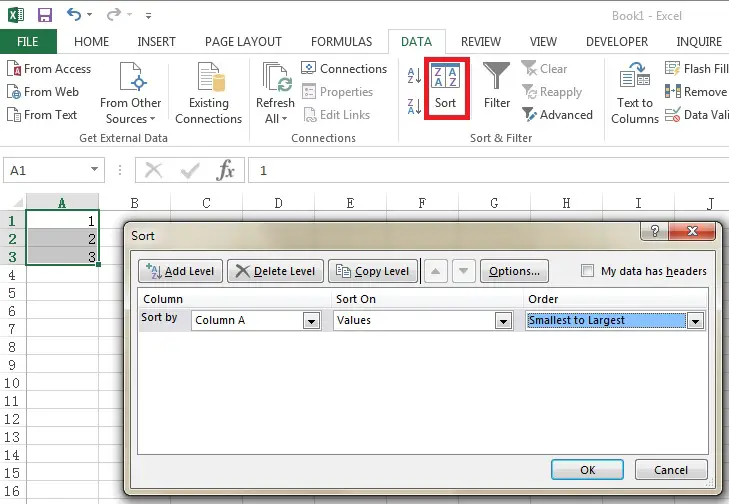
3 – Use sort Function as seen below, which is a Range Method in VBA.


excel_sort


Syntax of Excel Range Sort Method


Range .Sort(Key1, Order1, Key2, Type, Order2, Key3, Order3, Header, OrderCustom, MatchCase, Orientation, SortMethod, DataOption1, DataOption2, DataOption3)


Example of Excel Range Sort Method using dynamic range


Although there are so many arguments in Range Sort Method,  you only need to use four arguments for basic sorting:  Key, Order, Orientation, Header.


Because you will need to define a Range for Sort Method but the number of rows may vary, the below example defines the last row in column A as lastRow variable.


The below example shows how to sort column A and B, with column A in ascending order and column B in descending order.


Public Sub test_sort()
    lastRow = Range("A" & Rows.Count).End(xlUp).Row
    Set Rng = Range("A1:B" & lastRow)
    With Rng
        .Sort Key1:=.Range("A1"), Order1:=xlAscending, _
              Key2:=.Range("B1"), Order2:=xlAscending, Orientation:=xlSortColumns, _
              Header:=xlYes
    End With
End Sub

If you read carefully the description of argument Key1, it says “first sort field”. Some people interpret it is as the first Cell to sort, but according to my testing, if you input a Range such as A2, Excel only takes the column letter you input, but neglect the row number, therefore you can type A2, A3 or even A10000.


Outbound References


https://msdn.microsoft.com/en-us/library/microsoft.office.interop.excel.range.sort.aspx


Excel Range Sort Method to sort data
NameRequired/OptionalData TypeDescription
Key1OptionalVariantSpecifies the first sort field, either as a range name (String) or Range object; determines the values to be sorted.
Order1OptionalXlSortOrderDetermines the sort order for the values specified in Key1.


xlAscending (default)
xlDescending
Key2OptionalVariantSecond sort field; cannot be used when sorting a pivot table.
TypeOptionalVariantSpecified whether to sort Label or Values when sorting Pivot Report.


xlSortLabels
xlSortValues

Order2OptionalXlSortOrderDetermines the sort order for the values specified in Key2.


xlAscending (default)
xlDescending
Key3OptionalVariantThird sort field; cannot be used when sorting a pivot table.
Order3OptionalXlSortOrderDetermines the sort order for the values specified in Key3.


xlAscending (default)
xlDescending
HeaderOptionalXlYesNoGuessSpecifies whether the first row contains header information.


XlNo (Default)No header
XlYesHas header
XlGuessGuess has header or not
OrderCustomOptionalVariantSpecifies a one-based integer offset into the list of custom sort orders.
MatchCaseOptionalVariantSet to True to perform a case-sensitive sort, False to perform non-case sensitive sort; cannot be used with pivot tables.
OrientationOptionalXlSortOrientationSpecifies if the sort should by row or column


xlSortRows (default)
xlSortColumns

SortMethodOptionalXlSortMethodSpecifies the sort method of Chinese


xlStrokeSorting by the quantity of strokes in each character
xlPinYin (default)Phonetic Chinese sort order for characters
DataOption1OptionalXlSortDataOptionSpecifies how to sort text in the range specified in Key1; does not apply to pivot table sorting.


xlSortTextAsNumbersTreats text as numeric data for the sort.
xlSortNormal (default)Sorts numeric and text data separately.

DataOption2OptionalXlSortDataOptionSpecifies how to sort text in the range specified in Key2; does not apply to pivot table sorting.


xlSortTextAsNumbersTreats text as numeric data for the sort.
xlSortNormal (default)Sorts numeric and text data separately.

DataOption3OptionalXlSortDataOptionSpecifies how to sort text in the range specified in Key3; does not apply to pivot table sorting.


xlSortTextAsNumbersTreats text as numeric data for the sort.
xlSortNormal (default)Sorts numeric and text data separately.

2015年4月13日 星期一

Excel find all external links and broken links in workbook

This Excel tutorial explains how to find all external links and broken links in workbook using Find and Replace, Relationship Diagram, Macro.


You may also want to read


Excel VBA Workbook LinkSources Method


Excel VBA refresh closed workbook


Excel find all external links and broken links in workbook


There are several ways to find external links and broken links in workbook, some are easy to use but have limitations, I will talk about each method in this article. Note that this article writes about file link, not Hyperlink.


asktoupdatelinks


Basically there are three cases you would use external links:


1) In a formula, directly retrieve linked value


2) In a formula, retrieve value of Named Range defined in this workbook (simply go to Formulas > Name Manager to check)


3) In a formula, retrieve value of Named Range defined in external workbook


Less common use of external links include Objects and graphs. I am not going to talk about these less popular ones in this tutorial, you can click here to find out more from Microsoft support.


Use Find and Replace to find all external links


Normally, if you link a workbook to external source, you will see something like this in formula


='C:\Users\WYMAN\Desktop\folder\[FileB.xlsx]Sheet1'!$A$1

External links always refer to a another file name within square brackets [ ], we can make use of this characteristics and search the any string within workbook that contains [ or ], but the assumption is that you don’t actually have a text that contains square brackets.


Although you may think this is a ridiculous method, it is suggested by Microsoft. In fact, Excel maintains a dependency table for the links instead of just looking for the square brackets.


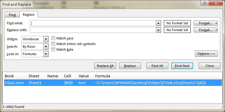
Press CTRL+F > input and select details as follows > Find all


broken_links


Now you can see all external links in the result box.


broken_links_02


This method cannot search Named Range defined in another workbook because [ ] are not present in the formula.


This method also fails to indicate broken links.


Use Cell Relationship Diagram to find all external links and broken links in workbook


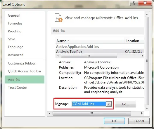
Excel 2013 introduces a new add-in to view the relationship diagram. To activate the add-in, navigate to Files > Options > Add-Ins


In dropdown box, select COM Add-ins > Press Go


broken_links_04


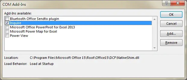
Select Inquire > Press OK


broken_links_05


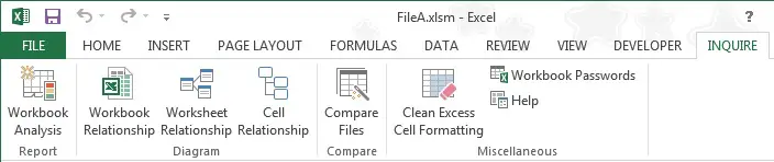
Now you have a new tab INQUIRE


broken_links_06


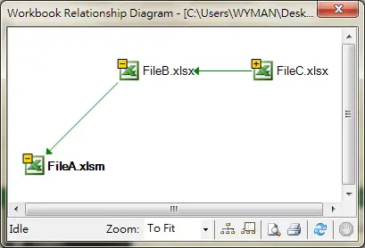
Workbook Relationship shows how your workbook is connected to other workbooks


broken_links_07


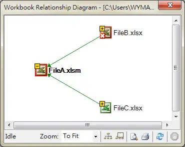
If workbook link is broken, you will find the Excel logo turns red


broken_links_10


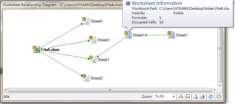
Worksheet Relationship shows how your worksheets are connect to other worksheets, it can also show the linked workbook information.


Similar to Workbook Relationship, you will also see the Excel logo turns red if the link is broken.


broken_links_08


Cell Relationship is relatively useless for our topic because it can only find the linked references for a single Cell each time.


Use Excel VBA to find all external links in workbook


If you only want to look for links used in formula, I highly recommend this VBA approach to you.


Excel has a workbook Method called LinkSources, which can be used to find the external workbook path+name.


For example,


C:\Users\WYMAN\Desktop\folder\FileB.xlsx

Although it fails to locate the Cell address that contains this path, we can loop through each used Range to find which one contains formula with this path to determine if the Cell contains a link.


As mentioned above, the external links can have square brackets or without square brackets, my Sub Procedures will take both into consideration in searching.


For example,


C:\Users\WYMAN\Desktop\folder\FileB.xlsx and C:\Users\WYMAN\Desktop\folder\[FileB.xlsx]

Use Excel VBA to find broken links


We can use Workbook LinkInfo Method to check status of each workbook.


Syntax of LinkInfo


Workbook.LinkInfo(Name, LinkInfo, Type, EditionRef)


NameRequired/OptionalData TypeDescription
NameRequiredStringThe name of the link.
LinkInfoRequiredXlLinkInfoThe type of information to be returned.


NameValueDescription
xlEditionDate2Applies only to editions in the Macintosh operating system.
xlLinkInfoStatus3Returns the link status.
xlUpdateState1Specifies whether the link updates automatically or manually.
TypeOptionalVariantOne of the constants of XlLinkInfoType specifying the type of link to return.


NameValueDescription
xlLinkInfoOLELinks2OLE or DDE server
xlLinkInfoPublishers5Publisher
xlLinkInfoSubscribers6Subscriber
EditionRefOptionalVariantIf the link is an edition, this argument specifies the edition reference as a string in R1C1 style. This argument is required if there’s more than one publisher or subscriber with the same name in the workbook.

LinkInfo Method returns a status as below.


XlLinkStatusDescription
xlLinkStatusCopiedValuesCopied values.
xlLinkStatusIndeterminateUnable to determine status.
xlLinkStatusInvalidNameInvalid name.
xlLinkStatusMissingFileFile missing.
xlLinkStatusMissingSheetSheet missing.
xlLinkStatusNotStartedNot started.
xlLinkStatusOKNo errors.
xlLinkStatusOldStatus may be out of date.
xlLinkStatusSourceNotCalculatedNot yet calculated.
xlLinkStatusSourceNotOpenNot open.
xlLinkStatusSourceOpenSource document is open.

Because the Method returns a number instead of XlLinkStatus, I need to create another Function linkStatusDescr to convert the XlLinkStatus to Description.


VBA code – find all external links and broken links in workbook


The below Procedure makes use of both LinkSources and LinkInfo Methods to find all external links and broken links in workbook.


Sub listLinks()
    aLinks = ActiveWorkbook.LinkSources(xlExcelLinks)
    If Not IsEmpty(aLinks) Then
        Sheets.Add
        shtName = ActiveSheet.Name
        Set summaryWS = ThisWorkbook.Worksheets(shtName)
        summaryWS.Range("A1") = "Worksheet"
        summaryWS.Range("B1") = "Cell"
        summaryWS.Range("C1") = "Formula"
        summaryWS.Range("D1") = "Workbook"
        summaryWS.Range("E1") = "Link Status"
        For Each Ws In ThisWorkbook.Worksheets
            If Ws.Name <> summaryWS.Name Then
                For Each rng In Ws.UsedRange
                    If rng.HasFormula Then
                        For j = LBound(aLinks) To UBound(aLinks)
                            linkStr = Left(aLinks(j), InStrRev(aLinks(j), "\")) & "[" & Right(aLinks(j), Len(aLinks(j)) - InStrRev(aLinks(j), "\"))
                            If InStr(rng.Formula, linkStr) Or InStr(rng.Formula, aLinks(j)) Then
                                lastRow = summaryWS.Range("A" & Rows.Count).End(xlUp).Row
                                summaryWS.Range("A" & lastRow + 1) = Ws.Name
                                summaryWS.Range("B" & lastRow + 1) = rng.Address
                                summaryWS.Range("C" & lastRow + 1) = "'" & rng.Formula
                                summaryWS.Range("D" & lastRow + 1) = aLinks(j)
                                summaryWS.Range("E" & lastRow + 1) = linkStatusDescr(ActiveWorkbook.LinkInfo(CStr(aLinks(j)), xlLinkInfoStatus))
                            End If
                        Next j
                    End If
                Next rng
            End If
        Next
    Else
        MsgBox "No external links"
    End If
    Columns("A:E").EntireColumn.AutoFit
End Sub

Public Function linkStatusDescr(statusCode)
           Select Case statusCode
                Case xlLinkStatusCopiedValues
                    linkStatusDescr = "Copied values"
                Case xlLinkStatusIndeterminate
                    linkStatusDescr = "Unable to determine status"
                Case xlLinkStatusInvalidName
                    linkStatusDescr = "Invalid name"
                Case xlLinkStatusMissingFile
                    linkStatusDescr = "File missing"
                Case xlLinkStatusMissingSheet
                    linkStatusDescr = "Sheet missing"
                Case xlLinkStatusNotStarted
                    linkStatusDescr = "Not started"
                Case xlLinkStatusOK
                    linkStatusDescr = "No errors"
                Case xlLinkStatusOld
                    linkStatusDescr = "Status may be out of date"
                Case xlLinkStatusSourceNotCalculated
                    linkStatusDescr = "Source not calculated yet"
                Case xlLinkStatusSourceNotOpen
                    linkStatusDescr = "Source not open"
                Case xlLinkStatusSourceOpen
                    linkStatusDescr = "Source open"
                Case Else
                    linkStatusDescr = "Unknown status"
            End Select
End Function

Result


All external links and status are displayed in a new worksheet.


Note that only Cell formula are checked, not Object or Named Range created in this workbook.


broken_links_09


Excel find all external links and broken links in workbook

2015年4月12日 星期日

Excel VBA Workbook LinkSources Method to find external links

This Excel tutorial explains how to use Workbook LinksSources Method in Excel VBA to find all external links.


You may also want to read:


How to refresh all external data of closed workbook


Excel VBA Workbook LinkSources Method


LinkSources can be used to return an array of names of linked documents, editions, or DDE or OLE servers.


Assume that you have two formula that link to another workbook, for example


='C:\Users\WYMAN\Desktop\folder\[FileB.xlsx]Sheet3'!$A$3

='C:\Users\WYMAN\Desktop\folder\[FileC.xlsx]Sheet3'!$A$3

The returned array is


Array (1) : C:\Users\WYMAN\Desktop\folder\FileB.xlsx

Array (2) : C:\Users\WYMAN\Desktop\folder\FileC.xlsx

Note that only the file name is returned, not the actual Cell address.


Syntax of Workbook LinkSources


Workbook.LinkSources(Type)


NameRequired/OptionalDescription
TypeOptionalOne of the constants of XlLink which specifies the type of link to return.Return all types if Type is omitted.


NameValueDescription
xlExcelLinks1The link is to an Excel worksheet.
xlOLELinks2The link is to an OLE source.
xlPublishers5Macintosh only.
xlSubscribers6Macintosh only.

Example of Workbook LinkSources


The below code creates a new worksheet and list all external source name (workbook name).


Sub listLinks()
    Dim aLinks As Variant
    aLinks = ActiveWorkbook.LinkSources(xlExcelLinks)
    If Not IsEmpty(aLinks) Then
        Sheets.Add
        For i = 1 To UBound(aLinks)
            Cells(i, 1).Value = aLinks(i)
        Next i
    End If
End Sub

The below code update all links in workbook


ActiveWorkbook.UpdateLink Name:=ActiveWorkbook.LinkSources

Click here to see how to refresh external links of closed workbook.


Excel find all external links and broken links in workbook


The below code shows how to find all external links and broken links in workbook with status on each linked source.

Sub listLinks2()
    aLinks = ActiveWorkbook.LinkSources(xlExcelLinks)
    If Not IsEmpty(aLinks) Then
        Sheets.Add
        shtName = ActiveSheet.Name
        Set summaryWS = ThisWorkbook.Worksheets(shtName)
        summaryWS.Range("A1") = "Worksheet"
        summaryWS.Range("B1") = "Cell"
        summaryWS.Range("C1") = "Formula"
        summaryWS.Range("D1") = "Workbook"
        summaryWS.Range("E1") = "Link Status"
        For Each Ws In ThisWorkbook.Worksheets
            If Ws.Name <> summaryWS.Name Then
                For Each rng In Ws.UsedRange
                    If rng.HasFormula Then
                        For j = LBound(aLinks) To UBound(aLinks)
                            linkStr = Left(aLinks(j), InStrRev(aLinks(j), "\")) & "[" & Right(aLinks(j), Len(aLinks(j)) - InStrRev(aLinks(j), "\"))
                            If InStr(rng.Formula, linkStr) Or InStr(rng.Formula, aLinks(j)) Then
                                lastRow = summaryWS.Range("A" & Rows.Count).End(xlUp).Row
                                summaryWS.Range("A" & lastRow + 1) = Ws.Name
                                summaryWS.Range("B" & lastRow + 1) = rng.Address
                                summaryWS.Range("C" & lastRow + 1) = "'" & rng.Formula
                                summaryWS.Range("D" & lastRow + 1) = aLinks(j)
                                summaryWS.Range("E" & lastRow + 1) = linkStatusDescr(ActiveWorkbook.LinkInfo(CStr(aLinks(j)), xlLinkInfoStatus))
                            End If
                        Next j
                    End If
                Next rng
            End If
        Next
    Else
        MsgBox "No external links"
    End If
End Sub


Public Function linkStatusDescr(statusCode)
           Select Case statusCode
                Case xlLinkStatusCopiedValues
                    linkStatusDescr = "Copied values"
                Case xlLinkStatusIndeterminate
                    linkStatusDescr = "Unable to determine status"
                Case xlLinkStatusInvalidName
                    linkStatusDescr = "Invalid name"
                Case xlLinkStatusMissingFile
                    linkStatusDescr = "File missing"
                Case xlLinkStatusMissingSheet
                    linkStatusDescr = "Sheet missing"
                Case xlLinkStatusNotStarted
                    linkStatusDescr = "Not started"
                Case xlLinkStatusOK
                    linkStatusDescr = "No errors"
                Case xlLinkStatusOld
                    linkStatusDescr = "Status may be out of date"
                Case xlLinkStatusSourceNotCalculated
                    linkStatusDescr = "Source not calculated yet"
                Case xlLinkStatusSourceNotOpen
                    linkStatusDescr = "Source not open"
                Case xlLinkStatusSourceOpen
                    linkStatusDescr = "Source open"
                Case Else
                    linkStatusDescr = "Unknown status"
            End Select
End Function

Outbound References


https://msdn.microsoft.com/en-us/library/office/ff821922.aspx


Excel VBA Workbook LinkSources Method to find external links

2015年4月10日 星期五

Excel VBA refresh closed workbook

This Excel tutorial explains how to refresh a closed workbook.


Excel refresh closed workbook


First of all, to refresh closed workbook involves opening the workbook, refresh and then close it,  it is impossible to refresh closed workbook without opening it, but we can open a workbook by vba without seeing it physically opened.


This question was originally asked in Microsoft Community, I answered the question and moved it here with some modifications.


Excel VBA Code – refresh closed workbook


Public Sub refreshXLS()
    Dim fso As Object
    Dim folder As Object
    Dim file As Object
    Path = "C:\Users\WYMAN\Desktop\folder\"
    Set fso = CreateObject("Scripting.FileSystemObject")
    Set folder = fso.GetFolder(Path)
    
    With Application
        .DisplayAlerts = False
        .ScreenUpdating = False
        .EnableEvents = False
        .AskToUpdateLinks = False
    End With

    For Each file In folder.Files
        If Right(file.Name, 4) = "xlsx" Or Right(file.Name, 3) = "xls" Then
            Workbooks.Open Path & file.Name
            ActiveWorkbook.UpdateLink Name:=ActiveWorkbook.LinkSources
            ActiveWorkbook.Close True
         End If
    Next

        With Application
        .DisplayAlerts = True
        .ScreenUpdating = True
        .EnableEvents = True
        .AskToUpdateLinks = True
    End With
End Sub

Explanation of VBA Code – refresh closed workbook


At the beginning of the code, I disable DisplayALerts, ScreenUpdating, EnableEvents and AskToUpdateLinks, we need to make sure no message box is prompted to interrupt the refresh code.


The Sub Procedure loop through specific folder and find all xls and xlsx files.


For each workbook, open it and refresh all links, finally close the workbook.


As you open the workbook, you will be prompted to confirm if you want to update external source, Application.AskToUpdateLinks disable the message.


Application.ScreenUpdating allows you to update without seeing the workbook open and close.


Excel VBA refresh closed workbook

2015年4月9日 星期四

Excel VBA AskToUpdateLinks Property

This Excel tutorial explains how to enable and disable Application AskToUpdateLinks Property (Ask to update automatic links in Excel Options).


You may also want to read


Differences among Function, Sub, Method, Property


Excel Options – Ask to Update automatic links


When you link external data source outside your workbook, such as another workbook or Access database, you will be asked whether to update the data automatically when you open the workbook.


This workbook contains links to one or more external sources that could be unsafe.


If you trust the links, update them to get the latest data. Otherwise, you can keep working with the data you have.


asktoupdatelinks


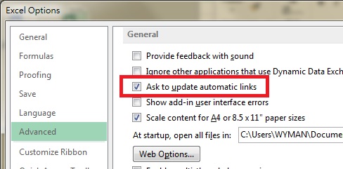
You can turn the message off in Excel Options > Advanced > Ask to update automatic links


asktoupdatelinks_02


Note that if you open the workbook which links back to a currently opened workbook, no message is prompted.


Excel VBA AskToUpdateLinks Property


When you programatically open the workbook with VBA, you need to make sure this option is off so that you can run Macro afterwards.


To make sure Ask to update automatic links Option is off, use Application Property AskToUpdateLinks as follows


Application.AskToUpdateLinks = False

To enable the option again, set the Property to True


Application.AskToUpdateLinks = True

However, user may have already turned it off by default, you don’t want to change their original setting after the Macro is run.


Since AskToUpdateLinks is a Property, which has a pair of Get and Set Methods, you can check if AskToUpdateLinks is set to True or False before you make that change, and restore the original setting when Macro is done.


Below is an example to open a workbook, disable AskToUpdateLinks and finally restore the user setting in the end.


Since AskToUpdateLinks is a global setting for all workbooks, you can check the user setting before target workbook is opened.


Public Sub openFile()
    userSetting = Application.AskToUpdateLinks
    Application.AskToUpdateLinks = False
    Set masterWB = Workbooks.Open("C:\Users\WYMAN\Desktop\folder\FileB.xlsx")
    'Run your Macro
    Application.AskToUpdateLinks = userSetting
End Sub

Outbound References


https://msdn.microsoft.com/zh-tw/library/office/ff194812%28v=office.14%29.aspx


Excel VBA AskToUpdateLinks Property

Excel VBA Function sum colored Cell count colored Cell

This Excel tutorial explains how to sum colored Cell and count colored Cell in Excel worksheet.


Excel VBA Function sum colored Cell and count colored cell


In my previous posts, I have explained how to use ColorIndex Property to find the first colored Cell. In this Post I will create a custom Function to count colored Cell of a Range and sum colored Cell


To recap the previous posts, you can click on the followings.


Excel VBA custom Function Find the first colored Cell value


VBA Excel ColorIndex Property


VBA Function Code – count colored Cell using ColorIndex Property


In the below Function, I use ColorIndex<>xlNone to identify colored Cell. White is deemed as colored, while “No Fill” is not colored.


If you just want to sum or count specific color, change the code


Interior.ColorIndex <> xlNone to Interior.ColorIndex = color_index (click here to see the list of color index)


Public Function wCountColorCell(rng As Range)
    Application.Volatile
    wCountColorCell = 0
    For Each r In rng
        If r.Interior.ColorIndex <> xlNone Then
            wCountColorCell = wCountColorCell+1
        End If
    Next r
End Function

Function Syntax – count colored Cell value using ColorIndex Property


wCountColorCell(rng)

rng is a Range that contains one more or Cells.


Function Example – count colored Cell value ColorIndex Property


Once you type a formula in Cell, the result cannot be refreshed automatically if you add/remove color to argument Range.


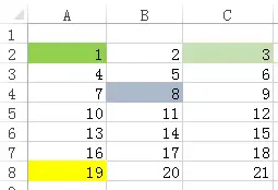
first_color_cell


FormulaResultExplanation
=wCountColorCell(A2:C2)2Count color Cell in the same row
=wCountColorCell(A2:A8)2Count color Cell in the same column
=wCountColorCell(A3:C8)2Count color Cell in the across different column and row

VBA Function Code – sum colored Cell using ColorIndex Property


In the below Function, I use ColorIndex<>xlNone to identify colored Cell. White is deemed as colored, while “No Fill” is not colored.


If you just want to sum or count specific color, change the code


Interior.ColorIndex <> xlNone to Interior.ColorIndex = color_index (click here to see the list of color index)


Public Function wSumColorCell(rng As Range)
    Application.Volatile
    wSumColorCell = 0
    For Each r In rng
        If r.Interior.ColorIndex <> xlNone Then
            wSumColorCell = wSumColorCell+r.Value
        End If
    Next r
End Function

Function Example – sum colored Cell using ColorIndex Property


Once you type a formula in Cell, the result cannot be refreshed automatically if you add/remove color to argument Range.


first_color_cell


FormulaResultExplanation
=wSumColorCell(A2:C2)4Sum color Cell in the same row
=wSumColorCell(A2:A8)20Sum color Cell in the same column
=wSumColorCell(A3:C8)27Sum color Cell in the across different column and row


Excel VBA Function sum colored Cell count colored Cell